Package: xcms
Authors: Philippine Louail, Johannes Rainer
Modified: 2026-04-22 09:50:36.294717
Compiled: Wed Apr 22 11:07:08 2026
Introduction
The xcms package provides the functionality to perform the preprocessing of LC-MS, GC-MS or LC-MS/MS data in which raw signals from mzML, mzXML or CDF files are processed into feature abundances. This preprocessing includes chromatographic peak detection, sample alignment and correspondence analysis.
The first version of the package was already published in 2006 [1] and has since been updated and modernized in several rounds to better integrate it with other R-based packages for the analysis of untargeted metabolomics data. This includes version 3 of xcms that used the MSnbase package for MS data representation [2]. The most recent update (xcms version 4) [3] enables in addition preprocessing of MS data represented by the modern MsExperiment and Spectra packages which provides an even better integration with the RforMassSpectrometry R package ecosystem simplifying e.g. also compound annotation [4].
This document describes data import, exploration and preprocessing of a simple test LC-MS data set with the xcms package version >= 4 [3]. The same functions can be applied to the older MSnbase-based workflows (xcms version 3). Additional documents and tutorials covering also other topics of untargeted metabolomics analysis are listed at the end of this document. An extensive collection of metabolomics data analysis tutorials, also including a complete end-to-end data analysis workflow as well as an example analysis of a very large-scale experiment using the new on-disk xcms result object is available at the Metabonaut website.
Preprocessing of LC-MS data
Data import
xcms supports analysis of any LC-MS(/MS) data that can be imported with the Spectra package. Such data will typically be provided in (AIA/ANDI) NetCDF, mzXML and mzML format but can, through dedicated extensions to the Spectra package, also be imported from other sources, e.g. also directly from raw data files in manufacturer’s formats.
For demonstration purpose we will analyze in this document a small subset of the data from [5] in which the metabolic consequences of the knock-out of the fatty acid amide hydrolase (FAAH) gene in mice was investigated. The raw data files (in NetCDF format) are provided through the faahKO data package. The data set consists of samples from the spinal cords of 6 knock-out and 6 wild-type mice. Each file contains data in centroid mode acquired in positive ion polarity from 200-600 m/z and 2500-4500 seconds. To speed-up processing of this vignette we will restrict the analysis to only 8 files.
Below we load all required packages, locate the raw CDF files within
the faahKO package and build a phenodata
data.frame describing the experimental setup. Generally,
such data frames should contain all relevant experimental variables and
sample descriptions (including also the names of the raw data files) and
will be imported into R using either the read.table()
function (if the file is in csv or tabulator delimited text
file format) or also using functions from the readxl R package
if it is in Excel file format.
library(xcms)
library(faahKO)
library(RColorBrewer)
library(pander)
library(pheatmap)
library(MsExperiment)

## Get the full path to the CDF files
cdfs <- dir(system.file("cdf", package = "faahKO"), full.names = TRUE,
            recursive = TRUE)[c(1, 2, 5, 6, 7, 8, 11, 12)]
## Create a phenodata data.frame
pd <- data.frame(sample_name = sub(basename(cdfs), pattern = ".CDF",
                                   replacement = "", fixed = TRUE),
                 sample_group = c(rep("KO", 4), rep("WT", 4)),
                 stringsAsFactors = FALSE)
We next load our data using the readMsExperiment
function from the MsExperiment
package.
faahko <- readMsExperiment(spectraFiles = cdfs, sampleData = pd)
faahko
## Object of class MsExperiment
## Spectra: MS1 (10224)
## Experiment data: 8 sample(s)
## Sample data links:
## - spectra: 8 sample(s) to 10224 element(s).The MS spectra data from our experiment is now available as a
Spectra object within faahko. Note that this
MsExperiment container could in addition to spectra data
also contain other types of data or also references to other files. See
the vignette from the MsExperiment
for more details. Also, when loading data from mzML, mzXML or CDF files,
by default only general spectra data is loaded into memory while the
actual peaks data, i.e. the m/z and intensity values are only
retrieved on-the-fly from the raw files when needed (this is similar to
the MSnbase on-disk mode described in [2]). This guarantees a low memory footprint
hence allowing to analyze also large experiments without the need of
high performance computing environments. Note that also different
alternative backends (and hence data representations) could be
used for the Spectra object within faahko with
eventually even lower memory footprint, or higher performance. See the
package vignette from the Spectra
package or the SpectraTutorials
tutorial for more details on Spectra backends and how to
change between them.
Initial data inspection
The MsExperiment object is a simple and flexible
container for MS experiments. The raw MS data is stored as a
Spectra object that can be accessed through the
spectra() function.
spectra(faahko)## MSn data (Spectra) with 10224 spectra in a MsBackendMzR backend:
## msLevel rtime scanIndex
## <integer> <numeric> <integer>
## 1 1 2501.38 1
## 2 1 2502.94 2
## 3 1 2504.51 3
## 4 1 2506.07 4
## 5 1 2507.64 5
## ... ... ... ...
## 10220 1 4493.56 1274
## 10221 1 4495.13 1275
## 10222 1 4496.69 1276
## 10223 1 4498.26 1277
## 10224 1 4499.82 1278
## ... 34 more variables/columns.
##
## file(s):
## ko15.CDF
## ko16.CDF
## ko21.CDF
## ... 5 more filesAll spectra are organized sequentially (i.e., not by file)
but the fromFile() function can be used to get for each
spectrum the information to which of the data files it belongs. Below we
simply count the number of spectra per file.
##
##    1    2    3    4    5    6    7    8
## 1278 1278 1278 1278 1278 1278 1278 1278
Information on samples can be retrieved through the
sampleData() function.
sampleData(faahko)## DataFrame with 8 rows and 3 columns
## sample_name sample_group spectraOrigin
## <character> <character> <character>
## ko15.CDF ko15 KO /__w/_temp...
## ko16.CDF ko16 KO /__w/_temp...
## ko21.CDF ko21 KO /__w/_temp...
## ko22.CDF ko22 KO /__w/_temp...
## wt15.CDF wt15 WT /__w/_temp...
## wt16.CDF wt16 WT /__w/_temp...
## wt21.CDF wt21 WT /__w/_temp...
## wt22.CDF wt22 WT /__w/_temp...Each row in this DataFrame represents one sample (input
file). Using [ it is possible to subset a
MsExperiment object by sample. Below we
subset the faahko to the 3rd sample (file) and access its
spectra and sample data.
faahko_3 <- faahko[3]
spectra(faahko_3)
## MSn data (Spectra) with 1278 spectra in a MsBackendMzR backend:
## msLevel rtime scanIndex
## <integer> <numeric> <integer>
## 1 1 2501.38 1
## 2 1 2502.94 2
## 3 1 2504.51 3
## 4 1 2506.07 4
## 5 1 2507.64 5
## ... ... ... ...
## 1274 1 4493.56 1274
## 1275 1 4495.13 1275
## 1276 1 4496.69 1276
## 1277 1 4498.26 1277
## 1278 1 4499.82 1278
## ... 34 more variables/columns.
##
## file(s):
## ko21.CDF
sampleData(faahko_3)## DataFrame with 1 row and 3 columns
## sample_name sample_group spectraOrigin
## <character> <character> <character>
## ko21.CDF ko21 KO /__w/_temp...As a first evaluation of the data we below plot the base peak
chromatogram (BPC) for each file in our experiment. We use the
chromatogram() method and set the
aggregationFun to "max" to return for each
spectrum the maximal intensity and hence create the BPC from the raw
data. To create a total ion chromatogram we could set
aggregationFun to "sum".
## Get the base peak chromatograms. This reads data from the files.
bpis <- chromatogram(faahko, aggregationFun = "max")
## Define colors for the two groups
group_colors <- paste0(brewer.pal(3, "Set1")[1:2], "60")
names(group_colors) <- c("KO", "WT")

## Plot all chromatograms.
plot(bpis, col = group_colors[sampleData(faahko)$sample_group])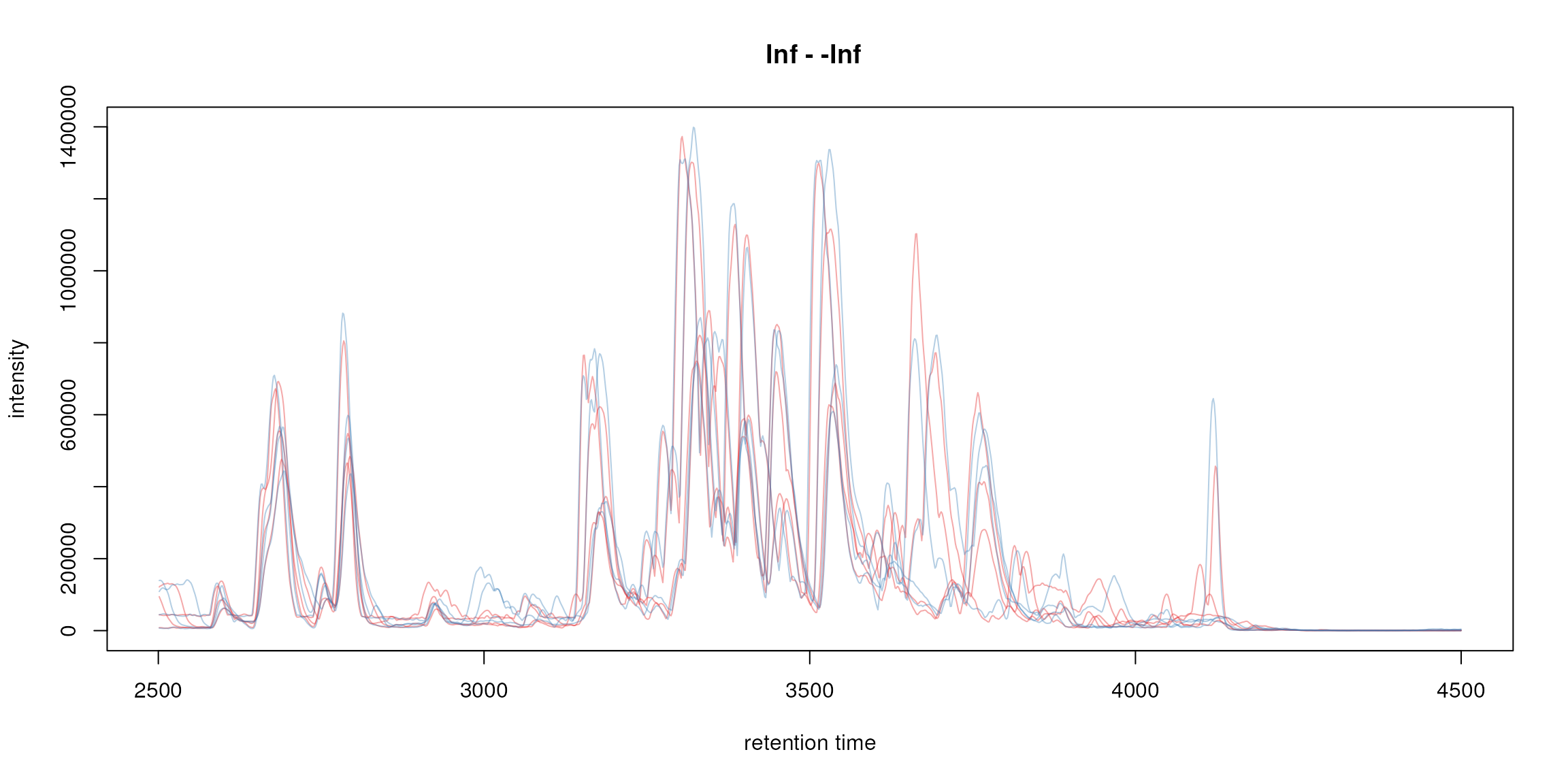
Base peak chromatogram.
The chromatogram() method returned a
MChromatograms object that organizes individual
Chromatogram objects (which in fact contain the
chromatographic data) in a two-dimensional array: columns represent
samples and rows (optionally) m/z and/or retention time ranges. Below we
extract the chromatogram of the first sample and access its retention
time and intensity values.
## [1] 2501.378 2502.943 2504.508 2506.073 2507.638 2509.203## [1] 43888 43960 43392 42632 42200 42288From the BPC above it seems that after around 4200 seconds no signal
is measured anymore. Thus, we filter below the full data set to a
retention time range from 2550 to 4250 seconds using the
filterRt() function. Note that at present this will only
subset the spectra within the MsExperiment. Subsequently we
re-create also the BPC.
faahko <- filterRt(faahko, rt = c(2550, 4250))
## creating the BPC on the subsetted data
bpis <- chromatogram(faahko, aggregationFun = "max")
We next create boxplots representing the distribution of the total
ion currents per data file. Such plots can be very useful to spot
potentially problematic MS runs. To extract this information, we use the
tic() function on the Spectra object within
faahko and split the values by file using
fromFile().
## Get the total ion current by file
tc <- spectra(faahko) |>
    tic() |>
    split(f = fromFile(faahko))
boxplot(tc, col = group_colors[sampleData(faahko)$sample_group],
        ylab = "intensity", main = "Total ion current")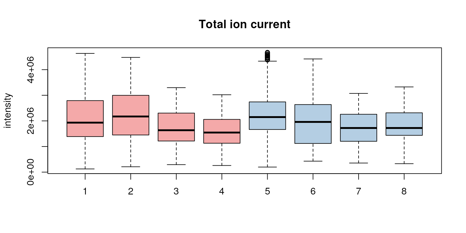
Distribution of total ion currents per file.
In addition, we can also cluster the samples based on similarity of
their base peak chromatograms. Samples would thus be grouped based on
similarity of their LC runs. For that we need however to bin
the data along the retention time axis, since retention times will
generally differ between samples. Below we use the bin()
function on the BPC to bin intensities into 2 second wide retention time
bins. The clustering is then performed using complete linkage
hierarchical clustering on the pairwise correlations of the binned base
peak chromatograms.
## Bin the BPC
bpis_bin <- bin(bpis, binSize = 2)

## Calculate correlation on the log2 transformed base peak intensities
cormat <- cor(log2(do.call(cbind, lapply(bpis_bin, intensity))))
colnames(cormat) <- rownames(cormat) <- bpis_bin$sample_name

## Define which phenodata columns should be highlighted in the plot
ann <- data.frame(group = bpis_bin$sample_group)
rownames(ann) <- bpis_bin$sample_name

## Perform the cluster analysis
pheatmap(cormat, annotation = ann,
         annotation_color = list(group = group_colors))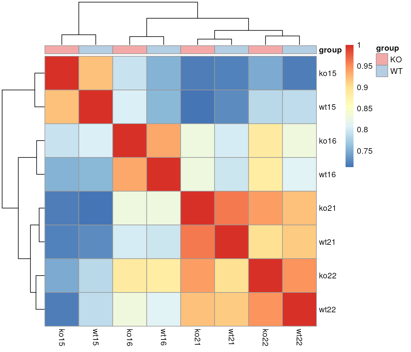
Grouping of samples based on similarity of their base peak chromatogram.
The samples cluster in a pairwise manner, with the KO and WT samples for the same sample index having the most similar BPC.
Chromatographic peak detection
Chromatographic peak detection aims at identifying all signal in each
sample created from ions of the same originating compound species.
Chromatographic peak detection can be performed in xcms with
the findChromPeaks() function and a parameter
object which defines and configures the algorithm that should be used
(see ?findChromPeaks for a list of supported algorithms).
Before running any peak detection it is however strongly suggested to
first visually inspect the extracted ion chromatogram of e.g. internal
standards or compounds known to be present in the samples in order to
evaluate and adapt the settings of the peak detection algorithm since
the default settings will not be appropriate for most LC-MS setups.
Below we extract the EIC for one compound using the
chromatogram() function by specifying in addition the m/z
and retention time range where we would expect the signal for that
compound.
## Define the rt and m/z range of the peak area
rtr <- c(2700, 2900)
mzr <- c(334.9, 335.1)
## extract the chromatogram
chr_raw <- chromatogram(faahko, mz = mzr, rt = rtr)
plot(chr_raw, col = group_colors[chr_raw$sample_group])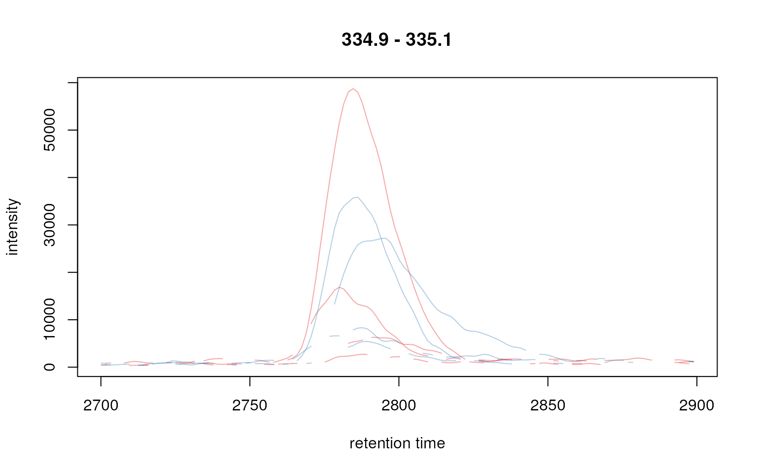
Extracted ion chromatogram for one peak.
Note that Chromatogram objects extracted by the
chromatogram() method contain an NA value if
in a certain scan (i.e. in a spectrum for a specific retention time) no
signal was measured in the respective m/z range. This is reflected by
the lines not being drawn as continuous lines in the plot above.
The peak above has thus a width of about 50 seconds. We can use this
information to define the peakwidth parameter of the
centWave peak detection method [6] that we will use for chromatographic peak
detection on our data. The peakwidth parameter allows to
define the expected lower and upper width (in retention time dimension)
of chromatographic peaks. For our data we set it thus to
peakwidth = c(20, 80). The second important parameter for
centWave is ppm which defines the expected maximum
deviation of m/z values of the centroids that should be included into
one chromatographic peak (note that this is not the
precision of m/z values provided by the MS instrument manufacturer).
For the ppm parameter we extract the full MS data
(intensity, retention time and m/z values) corresponding to the above
peak. To this end we first filter the raw object by retention time, then
by m/z and finally plot the object with type = "XIC" to
produce the plot below. We use the pipe (|>)
operator to better illustrate the corresponding workflow.
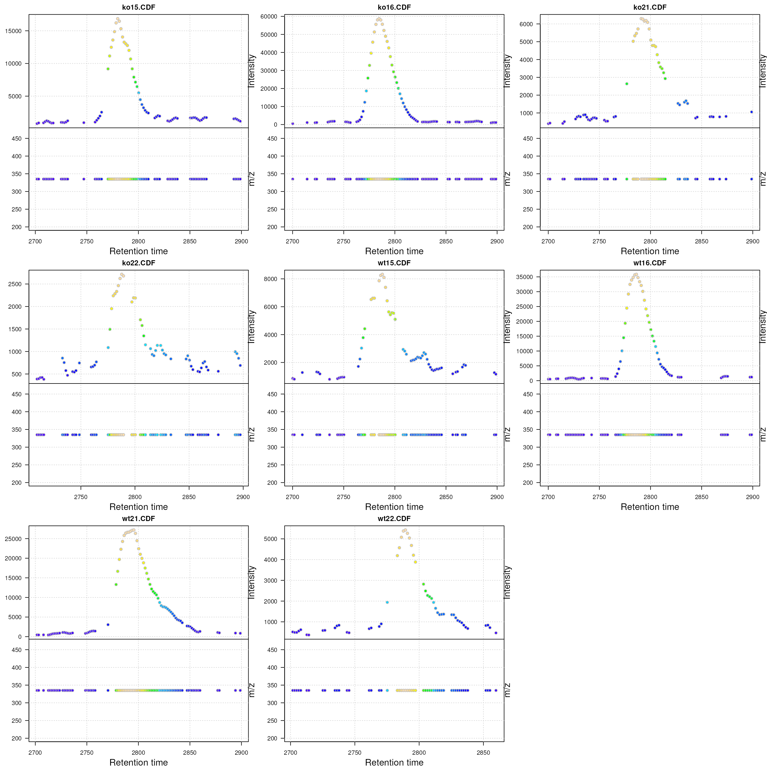
Visualization of the raw MS data for one peak. For each plot: upper panel: chromatogram plotting the intensity values against the retention time, lower panel m/z against retention time plot. The individual data points are colored according to the intensity.
In the present data there is actually no variation in the m/z values. Usually the m/z values of the individual centroids (lower panel) in the plots above would scatter around the real m/z value of the compound (in an intensity dependent manner).
The first step of the centWave algorithm defines regions
of interest (ROI) that are subsequently screened for the presence
of chromatographic peaks. These ROIs are defined based on the difference
of m/z values of centroids from consecutive scans (spectra). In detail,
centroids from consecutive scans are included into a ROI if the
difference between their m/z and the mean m/z of the ROI is smaller than
the user defined ppm parameter. A reasonable choice for the
ppm could thus be the maximal m/z difference of data points
from neighboring scans/spectra that are part of a chromatographic peak
for an internal standard of known compound. It is suggested to inspect
the ranges of m/z values for several compounds (either internal
standards or compounds known to be present in the sample) and define the
ppm parameter for centWave according to these. See
also this tutorial for
additional information and examples on choosing and testing peak
detection settings.
Chromatographic peak detection can also be performed on extracted ion
chromatograms, which helps testing and tuning peak detection settings.
Note however that peak detection on EICs does not involve the first step
of centWave described above and will thus not
consider the ppm parameter. Also, since less data is
available to the algorithms, background signal estimation is performed
differently and different settings for snthresh will need
to be used (generally a lower snthresh will be used for
EICs since the estimated background signal tends to be higher for data
subsets than for the full data). Below we perform the peak detection
with the findChromPeaks() function on the EIC generated
above. The submitted parameter object defines which algorithm
will be used and allows to define the settings for this algorithm. We
use a CentWaveParam parameter object to use and configure
the centWave algorithm with default settings, except for
snthresh.
xchr <- findChromPeaks(chr_raw, param = CentWaveParam(snthresh = 2))We can access the identified chromatographic peaks with the
chromPeaks() function.
chromPeaks(xchr)## mz mzmin mzmax rt rtmin rtmax into intb maxo
## mzmin 335 334.9 335.1 2781.505 2761.160 2809.674 412134.255 355516.374 16856
## mzmin 335 334.9 335.1 2786.199 2764.290 2812.803 1496244.206 1391821.332 58736
## mzmin 335 334.9 335.1 2734.556 2714.211 2765.855 21579.367 18449.428 899
## mzmin 335 334.9 335.1 2797.154 2775.245 2815.933 159058.782 150289.314 6295
## mzmin 335 334.9 335.1 2784.635 2761.160 2808.109 54947.545 37923.532 2715
## mzmin 335 334.9 335.1 2859.752 2845.668 2878.532 13895.212 13874.868 905
## mzmin 335 334.9 335.1 2897.311 2891.051 2898.876 5457.155 5450.895 995
## mzmin 335 334.9 335.1 2819.064 2808.109 2834.713 19456.914 19438.134 1347
## mzmin 335 334.9 335.1 2789.329 2762.725 2808.109 174473.311 91114.975 8325
## mzmin 335 334.9 335.1 2786.199 2764.290 2812.803 932645.211 569236.246 35856
## mzmin 335 334.9 335.1 2792.461 2768.987 2823.760 876585.527 511324.134 27200
## mzmin 335 334.9 335.1 2789.329 2773.680 2806.544 89582.569 73871.386 5427
## sn row column
## mzmin 13 1 1
## mzmin 20 1 2
## mzmin 4 1 3
## mzmin 12 1 3
## mzmin 2 1 4
## mzmin 904 1 4
## mzmin 994 1 4
## mzmin 1576 1 4
## mzmin 3 1 5
## mzmin 2 1 6
## mzmin 2 1 7
## mzmin 6 1 8Parallel to the chromPeaks() matrix there is also a
chromPeakData() data frame that allows to add arbitrary
annotations to each chromatographic peak, such as e.g. the MS level in
which the peak was detected:
chromPeakData(xchr)## DataFrame with 12 rows and 4 columns
## ms_level is_filled row column
## <integer> <logical> <integer> <integer>
## mzmin 1 FALSE 1 1
## mzmin 1 FALSE 1 2
## mzmin 1 FALSE 1 3
## mzmin 1 FALSE 1 3
## mzmin 1 FALSE 1 4
## ... ... ... ... ...
## mzmin 1 FALSE 1 4
## mzmin 1 FALSE 1 5
## mzmin 1 FALSE 1 6
## mzmin 1 FALSE 1 7
## mzmin 1 FALSE 1 8Below we plot the EIC along with all identified chromatographic peaks
using the plot() function on the result object from above.
Additional parameters peakCol and peakBg allow
to define a foreground and background (fill) color for each identified
chromatographic peak in the provided result object (i.e., we need to
define one color for each row of chromPeaks(xchr) - column
"column" (or "sample" if present) in that peak
matrix specifies the sample in which the peak was identified).
## Define a color for each sample
sample_colors <- group_colors[xchr$sample_group]
## Define the background color for each chromatographic peak
bg <- sample_colors[chromPeaks(xchr)[, "column"]]
## Parameter `col` defines the color of each sample/line, `peakBg` of each
## chromatographic peak.
plot(xchr, col = sample_colors, peakBg = bg)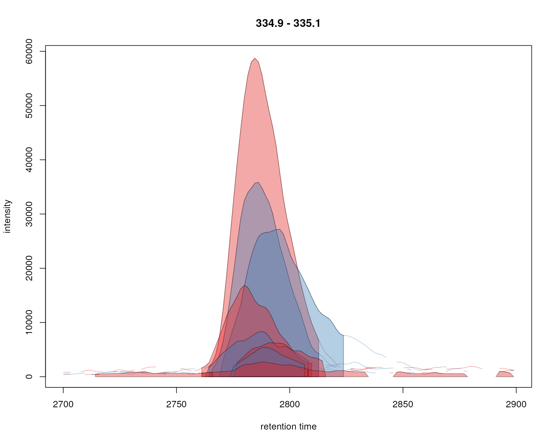
Signal for an example peak. Red and blue colors represent KO and wild type samples, respectively. Peak area of identified chromatographic peaks are highlighted in the sample group color.
If we are happy with the settings we can use them for the peak
detection on the full data set (i.e. on the MsExperiment
object with the data for the whole experiment). Note that below we set
the argument prefilter to c(6, 5000) and
noise to 5000 to reduce the run time of this
vignette. With this setting we consider only ROIs with at least 6
centroids with an intensity larger than 5000 for the centWave
chromatographic peak detection.
cwp <- CentWaveParam(peakwidth = c(20, 80), noise = 5000,
                     prefilter = c(6, 5000))
faahko <- findChromPeaks(faahko, param = cwp)
The results of findChromPeaks() on a
MsExperiment object are returned as an
XcmsExperiment object. This object extends
MsExperiment directly (hence providing the same access to
all raw data) and contains all xcms preprocessing results. Note
also that additional rounds of chromatographic peak detections could be
performed and their results being added to existing peak detection
results by additional calls to findChromPeaks() on the
result object and using parameter add = TRUE.
The chromPeaks function can also here be used to access
the results from the chromatographic peak detection. Below we show the
first 6 identified chromatographic peaks.
chromPeaks(faahko) |>
    head()
## mz mzmin mzmax rt rtmin rtmax into intb maxo sn
## CP0001 594.0 594.0 594.0 2601.535 2581.191 2637.529 161042.2 146073.3 7850 11
## CP0002 577.0 577.0 577.0 2604.665 2581.191 2626.574 136105.2 128067.9 6215 11
## CP0003 307.0 307.0 307.0 2618.750 2592.145 2645.354 284782.4 264907.0 16872 20
## CP0004 302.0 302.0 302.0 2617.185 2595.275 2640.659 687146.6 669778.1 30552 43
## CP0005 370.1 370.1 370.1 2673.523 2643.789 2700.127 449284.6 417225.3 25672 17
## CP0006 427.0 427.0 427.0 2675.088 2643.789 2684.478 283334.7 263943.2 11025 13
## sample
## CP0001 1
## CP0002 1
## CP0003 1
## CP0004 1
## CP0005 1
## CP0006 1Columns of this chromPeaks() matrix might differ
depending on the used peak detection algorithm. Columns that all
algorithms have to provide are: "mz", "mzmin",
"mzmax", "rt", "rtmin" and
"rtmax" that define the m/z and retention time range of the
chromatographic peak (i.e. all mass peaks within that area are used to
integrate the peak signal) as well as the m/z and retention time of the
peak apex. Other mandatory columns are "into" and
"maxo" with the absolute integrated peak signal and the
maximum peak intensity. Finally, "sample" provides the
index of the sample in which the peak was identified.
Additional annotations for each individual peak can be extracted with
the chromPeakData() function. This data frame could also be
used to add/store arbitrary annotations for each detected peak (that
don’t necessarily need to be numeric).
chromPeakData(faahko)## DataFrame with 2908 rows and 2 columns
## ms_level is_filled
## <integer> <logical>
## CP0001 1 FALSE
## CP0002 1 FALSE
## CP0003 1 FALSE
## CP0004 1 FALSE
## CP0005 1 FALSE
## ... ... ...
## CP2904 1 FALSE
## CP2905 1 FALSE
## CP2906 1 FALSE
## CP2907 1 FALSE
## CP2908 1 FALSEChromatographic peak quality
Based on the publication by Kumler et al. published in 2023 [7], new quality metrics (beta_cor and
beta_snr) were added to xcms. beta_cor
indicates how bell-shaped the chromatographic peak is and
beta_snr is estimating the signal-to-noise ratio using the
residuals from this fit. These metrics can be calculated during peak
picking by setting verboseBetaColumns = TRUE in the
CentWaveParam object, or they can be calculated afterwards
by using the chromPeakSummary() function with the
XcmsExperiment object and the
BetaDistributionParam parameter object as input:
beta_metrics <- chromPeakSummary(faahko, BetaDistributionParam())
head(beta_metrics)
## beta_cor beta_snr
## CP0001 0.9865868 5.349210
## CP0002 0.9401467 4.928835
## CP0003 0.9846982 5.783004
## CP0004 0.9883246 6.044377
## CP0005 0.6972246 5.293175
## CP0006 0.1358883 4.995241The result returned by chromPeakSummary() is thus a
numeric matrix with the values for these quality estimates, one row for
each chromatographic peak. Using summary statistics, one can explore the
distribution of these metrics in the data.
summary(beta_metrics)## beta_cor beta_snr
## Min. :-0.8541 Min. :3.921
## 1st Qu.: 0.7390 1st Qu.:5.157
## Median : 0.9442 Median :5.594
## Mean : 0.7904 Mean :5.662
## 3rd Qu.: 0.9771 3rd Qu.:6.097
## Max. : 0.9990 Max. :7.983
## NAs :6 NAs :6Visual inspection gives a better idea of what these metrics represent
in terms of peak quality in the data at hand. This information can be
used to e.g. filter out peaks that don’t meet a chosen quality metric
threshold. In order to plot the detected peaks, their EIC can be
extracted with the function chromPeakChromatograms. An
example of a peak with a high beta_cor and for a peak with a
low beta_cor score is given below.
beta_metrics[c(4, 6), ]## beta_cor beta_snr
## CP0004 0.9883246 6.044377
## CP0006 0.1358883 4.995241
eics <- chromPeakChromatograms(
    faahko, peaks = rownames(chromPeaks(faahko))[c(4, 6)])
Plots of high and low quality peaks. Left: peak CP0004 with a beta_cor = 0.98, right: peak CP0006 with a beta_cor = 0.13.
Refining peak detection
Peak detection will not always work perfectly for all types of peak
shapes present in the data set leading to peak detection artifacts, such
as (partially or completely) overlapping peaks or artificially split
peaks (common issues especially for centWave). xcms
provides the refineChromPeaks() function that can be called
on peak detection results in order to refine (or clean) peak
detection results by either removing identified peaks not passing a
certain criteria or by merging artificially split or partially or
completely overlapping chromatographic peaks. Different algorithms are
available that can again be configured with their respective parameter
objects: CleanPeaksParam and
FilterIntensityParam allow to remove peaks with their
retention time range or intensity being below a specified threshold,
respectively. With MergeNeighboringPeaksParam it is
possible to merge chromatographic peaks and hence remove many of the
above mentioned (centWave) peak detection artifacts. See also
?refineChromPeaks for more information and help on the
different methods.
Below we post-process the peak detection results merging peaks that
overlap in a 4 second window per file and for which the signal between
them is lower than 75% of the smaller peak’s maximal intensity. See the
?MergeNeighboringPeaksParam help page for a detailed
description of the settings and the approach.
mpp <- MergeNeighboringPeaksParam(expandRt = 4)
faahko_pp <- refineChromPeaks(faahko, mpp)
## Warning in rbindlistWithRownames(pkd_new, use.names = TRUE, fill = TRUE):
## Dropping rownames: duplicated rownames present or rownames not available for
## all data.frames
## Warning in rbindlistWithRownames(pkd_new, use.names = TRUE, fill = TRUE):
## Dropping rownames: duplicated rownames present or rownames not available for
## all data.frames## Warning in rbindlistWithRownames(lapply(res, `[[`, 2L), use.names = TRUE, :
## Dropping rownames: duplicated rownames present or rownames not available for
## all data.frames## Warning in rbindlistWithRownames(pkd_new, use.names = TRUE, fill = TRUE):
## Dropping rownames: duplicated rownames present or rownames not available for
## all data.frames
## Warning in rbindlistWithRownames(pkd_new, use.names = TRUE, fill = TRUE):
## Dropping rownames: duplicated rownames present or rownames not available for
## all data.frames
## Warning in rbindlistWithRownames(pkd_new, use.names = TRUE, fill = TRUE):
## Dropping rownames: duplicated rownames present or rownames not available for
## all data.frames
## Warning in rbindlistWithRownames(pkd_new, use.names = TRUE, fill = TRUE):
## Dropping rownames: duplicated rownames present or rownames not available for
## all data.frames
## Warning in rbindlistWithRownames(pkd_new, use.names = TRUE, fill = TRUE):
## Dropping rownames: duplicated rownames present or rownames not available for
## all data.frames
## Warning in rbindlistWithRownames(pkd_new, use.names = TRUE, fill = TRUE):
## Dropping rownames: duplicated rownames present or rownames not available for
## all data.frames## Warning in rbindlistWithRownames(lapply(res, `[[`, 2L)): Dropping rownames:
## duplicated rownames present or rownames not available for all data.framesAn example for a merged peak is given below.
mzr_1 <- 305.1 + c(-0.01, 0.01)
chr_1 <- chromatogram(faahko[1], mz = mzr_1)
chr_2 <- chromatogram(faahko_pp[1], mz = mzr_1)
par(mfrow = c(1, 2))
plot(chr_1)
plot(chr_2)
Result from the peak refinement step. Left: data before processing, right: after refinement. The splitted peak was merged into one.
centWave thus detected originally 3 chromatographic peaks in
the m/z slice (left panel in the plot above) and peak refinement with
MergeNeighboringPeaksParam and the specified settings
merged the first two peaks into a single one (right panel in the figure
above). Other close peaks, with a lower intensity between them, were
however not merged (see below).
mzr_1 <- 496.2 + c(-0.01, 0.01)
chr_1 <- chromatogram(faahko[1], mz = mzr_1)
chr_2 <- chromatogram(faahko_pp[1], mz = mzr_1)
par(mfrow = c(1, 2))
plot(chr_1)
plot(chr_2)
Result from the peak refinement step. Left: data before processing, right: after refinement. The peaks were not merged.
It is also possible to perform the peak refinement on extracted ion
chromatograms. This could again be used to test and fine-tune the
settings for the parameter and to avoid potential problematic behavior.
The minProp parameter for example has to be carefully
chosen to avoid merging of isomer peaks (like in the example above).
With the default minProp = 0.75 only peaks are merged if
the signal between the two peaks is higher than 75% of
the smaller peak’s maximal intensity. Setting this value too low could
eventually result in merging of isomers as shown below.
#' Too low minProp could cause merging of isomers!
res <- refineChromPeaks(chr_1, MergeNeighboringPeaksParam(minProp = 0.05))
chromPeaks(res)
## mz mzmin mzmax rt rtmin rtmax into intb maxo sn
## CPM1 496.2 496.19 496.21 3384.012 3294.809 3412.181 45940118 NA 1128960 177
## sample row column
## CPM1 1 1 1
plot(res)
Thus, before running such a peak refinement evaluate that isomers present in the data set were not wrongly merged based on the chosen settings.
Before proceeding we next replace the faahko object with
the results from the peak refinement step.
faahko <- faahko_ppBelow we use the data from the chromPeaks() matrix to
calculate per-file summaries of the peak detection results, such as the
number of peaks per file as well as the distribution of the retention
time widths.
summary_fun <- function(z)
    c(peak_count = nrow(z), rt = quantile(z[, "rtmax"] - z[, "rtmin"]))

T <- chromPeaks(faahko) |>
    split.data.frame(f = chromPeaks(faahko)[, "sample"]) |>
    lapply(FUN = summary_fun) |>
    do.call(what = rbind)
rownames(T) <- basename(fileNames(faahko))
pandoc.table(
    T,
    caption = paste0("Summary statistics on identified chromatographic",
                     " peaks. Shown are number of identified peaks per",
                     " sample and widths/duration of chromatographic ",
"peaks."))| peak_count | rt.0% | rt.25% | rt.50% | rt.75% | rt.100% | |
|---|---|---|---|---|---|---|
| ko15.CDF | 397 | 10.95 | 34.43 | 42.25 | 53.21 | 319.2 |
| ko16.CDF | 520 | 10.95 | 32.86 | 42.25 | 53.21 | 151.8 |
| ko21.CDF | 207 | 10.95 | 42.25 | 50.08 | 65.73 | 164.3 |
| ko22.CDF | 233 | 10.95 | 37.56 | 46.95 | 59.47 | 147.1 |
| wt15.CDF | 403 | 10.95 | 32.86 | 42.25 | 53.21 | 161.2 |
| wt16.CDF | 361 | 10.95 | 35.99 | 45.38 | 57.9 | 162.8 |
| wt21.CDF | 226 | 10.95 | 35.99 | 48.51 | 64.16 | 172.1 |
| wt22.CDF | 328 | 10.95 | 35.99 | 45.38 | 57.9 | 228.5 |
While by default chromPeaks() will return all identified
chromatographic peaks in a result object it is also possible to extract
only chromatographic peaks for a specified m/z and/or rt range:
chromPeaks(faahko, mz = c(334.9, 335.1), rt = c(2700, 2900))## mz mzmin mzmax rt rtmin rtmax into intb maxo sn
## CP0038 335 335 335 2781.505 2761.160 2809.674 412134.3 383167.4 16856 23
## CP0494 335 335 335 2786.199 2764.290 2812.803 1496244.2 1461187.3 58736 72
## CP1025 335 335 335 2797.154 2775.245 2815.933 159058.8 149229.6 6295 13
## CP1964 335 335 335 2786.199 2764.290 2812.803 932645.2 915333.8 35856 66
## CP2349 335 335 335 2792.461 2768.987 2823.760 876585.5 848569.1 27200 36
## sample
## CP0038 1
## CP0494 2
## CP1025 3
## CP1964 6
## CP2349 7We can also plot the location of the identified chromatographic peaks
in the m/z - retention time space for one file using the
plotChromPeaks() function. Below we plot this information
for the third sample.
plotChromPeaks(faahko, file = 3)
Identified chromatographic peaks in the m/z by retention time space for one sample.
As a general overview of the peak detection results we can in
addition visualize the number of identified chromatographic peaks per
file along the retention time axis. Parameter binSize
allows to define the width of the bins in rt dimension in which peaks
should be counted. This number of chromatographic peaks within each bin
is then shown color-coded in the resulting plot.
plotChromPeakImage(faahko, binSize = 10)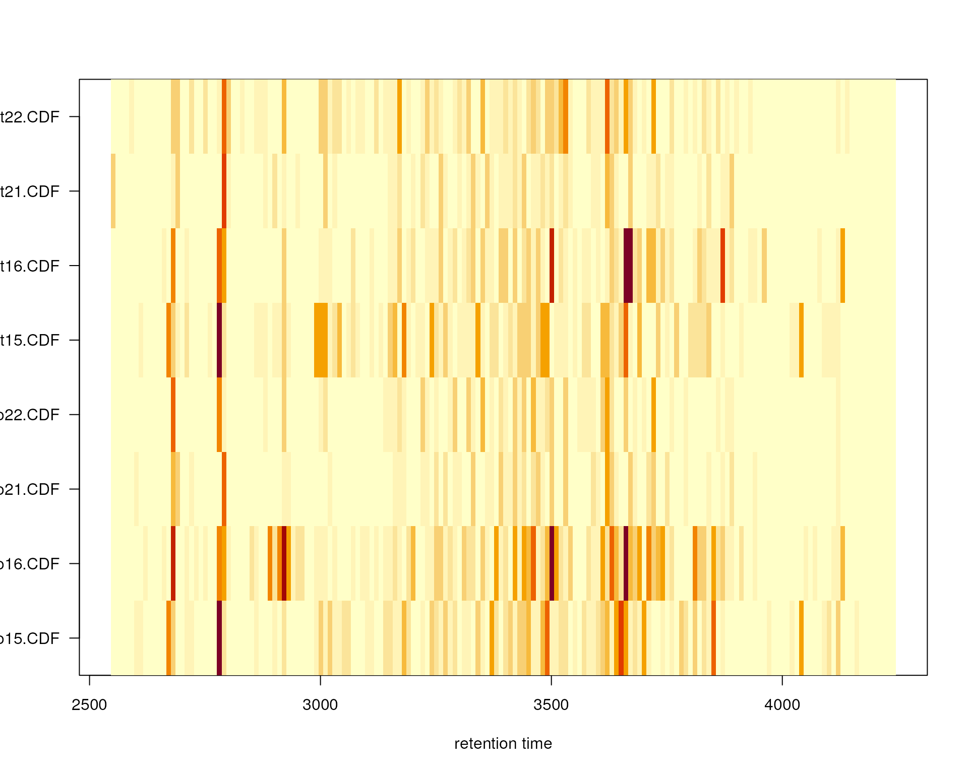
Frequency of identified chromatographic peaks along the retention time axis. The frequency is color coded with higher frequency being represented by yellow-white. Each line shows the peak frequency for one file.
Note that extracting ion chromatorams from an xcms result
object will in addition to the chromatographic data also extract any
identified chromatographic peaks within that region. This can thus also
be used to validate and verify that the used peak detection settings
identified e.g. peaks for known compounds or internal standards
properly. Below we extract the ion chromatogram for the m/z - rt region
above and access the detected peaks in that region using the
chromPeaks() function.
chr_ex <- chromatogram(faahko, mz = mzr, rt = rtr)
chromPeaks(chr_ex)
## mz mzmin mzmax rt rtmin rtmax into intb maxo sn
## CP0038 335 335 335 2781.505 2761.160 2809.674 412134.3 383167.4 16856 23
## CP0494 335 335 335 2786.199 2764.290 2812.803 1496244.2 1461187.3 58736 72
## CP1025 335 335 335 2797.154 2775.245 2815.933 159058.8 149229.6 6295 13
## CP1964 335 335 335 2786.199 2764.290 2812.803 932645.2 915333.8 35856 66
## CP2349 335 335 335 2792.461 2768.987 2823.760 876585.5 848569.1 27200 36
## sample row column
## CP0038 1 1 1
## CP0494 2 1 2
## CP1025 3 1 3
## CP1964 6 1 6
## CP2349 7 1 7We can also plot this extracted ion chromatogram which will also visualize all identified chromatographic peaks in that region.
sample_colors <- group_colors[chr_ex$sample_group]
plot(chr_ex, col = group_colors[chr_raw$sample_group], lwd = 2,
     peakBg = sample_colors[chromPeaks(chr_ex)[, "sample"]])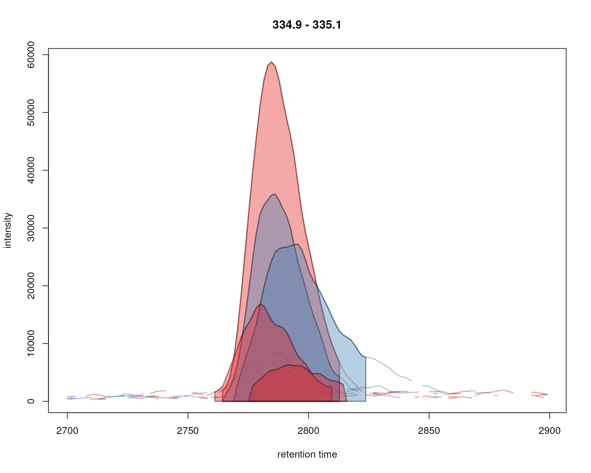
Signal for an example peak. Red and blue colors represent KO and wild type samples, respectively. The signal area of identified chromatographic peaks are filled with a color.
Chromatographic peaks can be visualized also in other ways: by
setting peakType = "rectangle" the they are indicated with
a rectangle instead of the default highlighting option
(peakType = "polygon") used above. As a third alternative
it would also possible to just indicate the apex position for each
identified chromatographic peak with a single point
(peakType = "point"). Below we plot the data again using
peakType = "rectangle".
plot(chr_ex, col = sample_colors, peakType = "rectangle",
     peakCol = sample_colors[chromPeaks(chr_ex)[, "sample"]],
     peakBg = NA)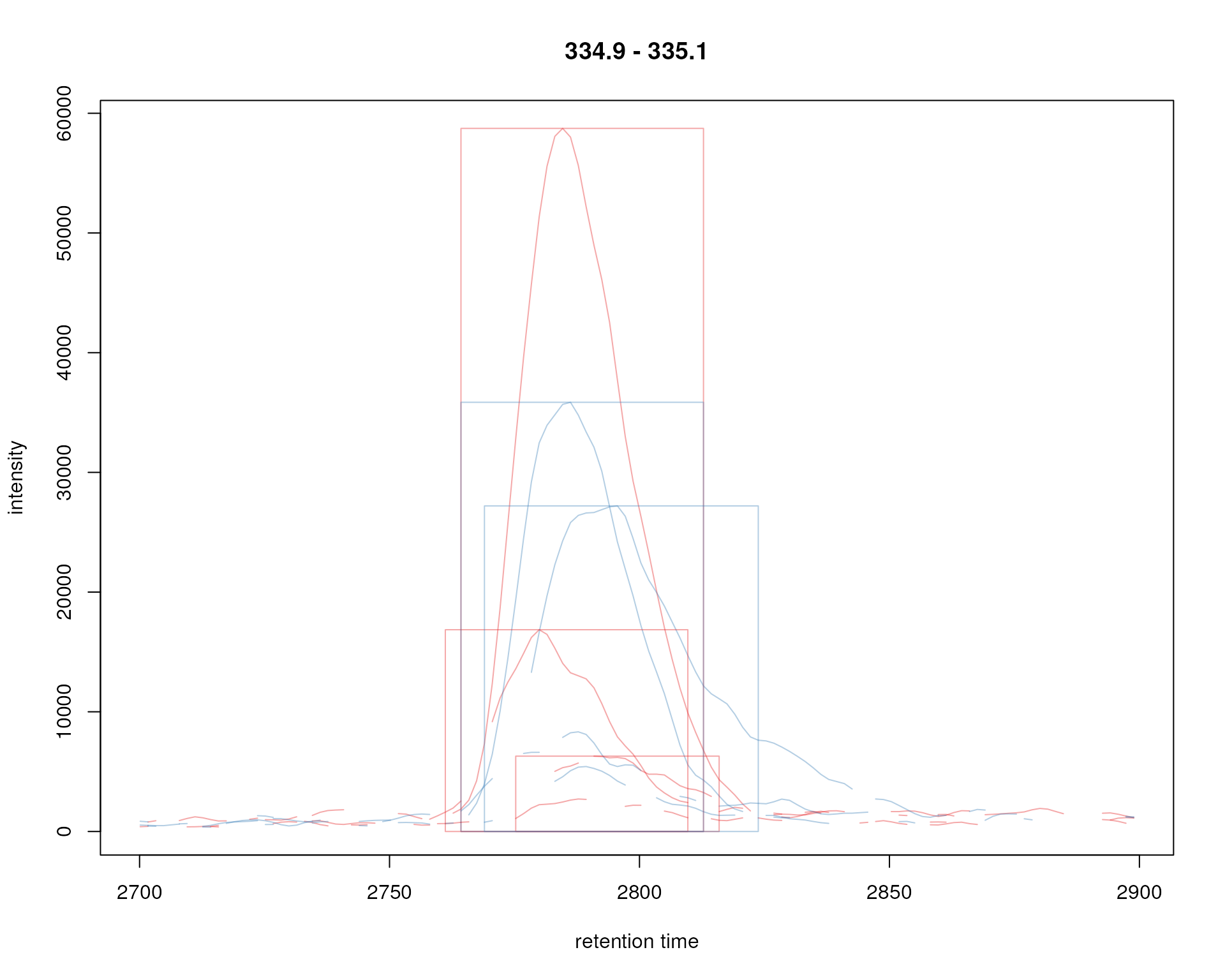
Signal for an example peak. Red and blue colors represent KO and wild type samples, respectively. The rectangles indicate the identified chromatographic peaks per sample.
Finally we plot also the distribution of peak intensity per sample. This allows to investigate whether systematic differences in peak signals between samples are present.
## Extract a list of per-sample peak intensities (in log2 scale)
ints <- split(log2(chromPeaks(faahko)[, "into"]),
              f = chromPeaks(faahko)[, "sample"])
boxplot(ints, varwidth = TRUE, col = sample_colors,
        ylab = expression(log[2]~intensity), main = "Peak intensities")
grid(nx = NA, ny = NULL)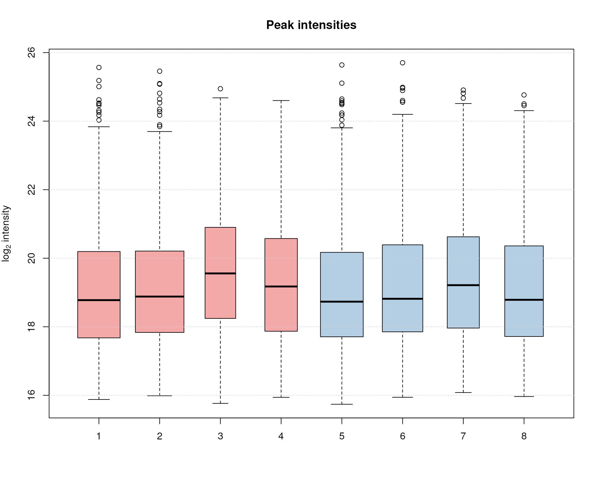
Peak intensity distribution per sample.
Over and above the signal of the identified chromatographic peaks is comparable across samples, with the exception of samples 3, 4 and, to some degree, also 7 that show slightly higher average intensities, but also a lower number of detected peaks (indicated by the smaller width of the boxes).
Note that in addition to the above described identification of
chromatographic peaks, it is also possible to manually define
and add chromatographic peaks with the manualChromPeaks()
function (see ?manualChromPeaks help page for more
information).
Alignment
The time at which analytes elute in the chromatography can vary between samples (and even compounds). Such differences were already visible in the BPC and even the extracted ion chromatogram plot in the previous section. The alignment step, also referred to as retention time correction, aims to adjust these differences by shifting signals along the retention time axis and aligning them between different samples within an experiment.
A plethora of alignment algorithms exist (see [8]), with some of them being also implemented
in xcms. Alignment of LC-MS data can be performed in
xcms using the adjustRtime() method and an
algorithm-specific parameter class (see ?adjustRtime for an
overview of available methods in xcms).
In the example below we use the obiwarp method [9] to align the samples. We use a
binSize = 0.6 which creates warping functions in m/z bins
of 0.6. Also here it is advisable to modify and adapt the settings for
each experiment.
faahko <- adjustRtime(faahko, param = ObiwarpParam(binSize = 0.6))Note that adjustRtime(), besides calculating adjusted
retention times for each spectrum, adjusts also the retention times of
the identified chromatographic peaks in the xcms result object.
Adjusted retention times of individual spectra can be extracted from the
result object using either the adjustedRtime() function or
using rtime() with parameter adjusted = TRUE
(the default):
## Extract adjusted retention times
adjustedRtime(faahko) |> head()
## [1] 2551.457 2553.089 2554.720 2556.352 2557.983 2559.615## [1] 2551.457 2553.089 2554.720 2556.352 2557.983 2559.615## [1] 2551.457 2553.022 2554.586 2556.151 2557.716 2559.281To evaluate the impact of the alignment we plot the BPC on the
adjusted data. In addition we plot also the differences between the
adjusted and the raw retention times per sample using the
plotAdjustedRtime() function. To disable the automatic
extraction of all identified chromatographic peaks by the
chromatogram() function (which would not make much sense
for a BPC) we use chromPeaks = "none" below.
## Get the base peak chromatograms.
bpis_adj <- chromatogram(faahko, aggregationFun = "max", chromPeaks = "none")
par(mfrow = c(3, 1), mar = c(4.5, 4.2, 1, 0.5))
plot(bpis, col = sample_colors)
grid()
plot(bpis_adj, col = sample_colors)
grid()
## Plot also the difference of adjusted to raw retention time.
plotAdjustedRtime(faahko, col = sample_colors)
grid()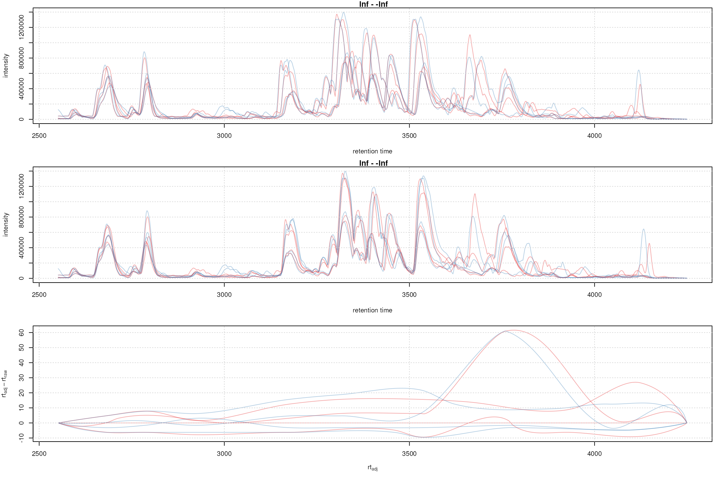
Obiwarp aligned data. Base peak chromatogram before (top) and after alignment (middle) and difference between adjusted and raw retention times along the retention time axis (bottom).
Too large differences between adjusted and raw retention times could indicate poorly performing samples or alignment.
At last we evaluate also the impact of the alignment on the test peak.
par(mfrow = c(2, 1))
## Plot the raw data
plot(chr_raw, col = sample_colors)
grid()
## Extract the chromatogram from the adjusted object
chr_adj <- chromatogram(faahko, rt = rtr, mz = mzr)
plot(chr_adj, col = sample_colors, peakType = "none")
grid()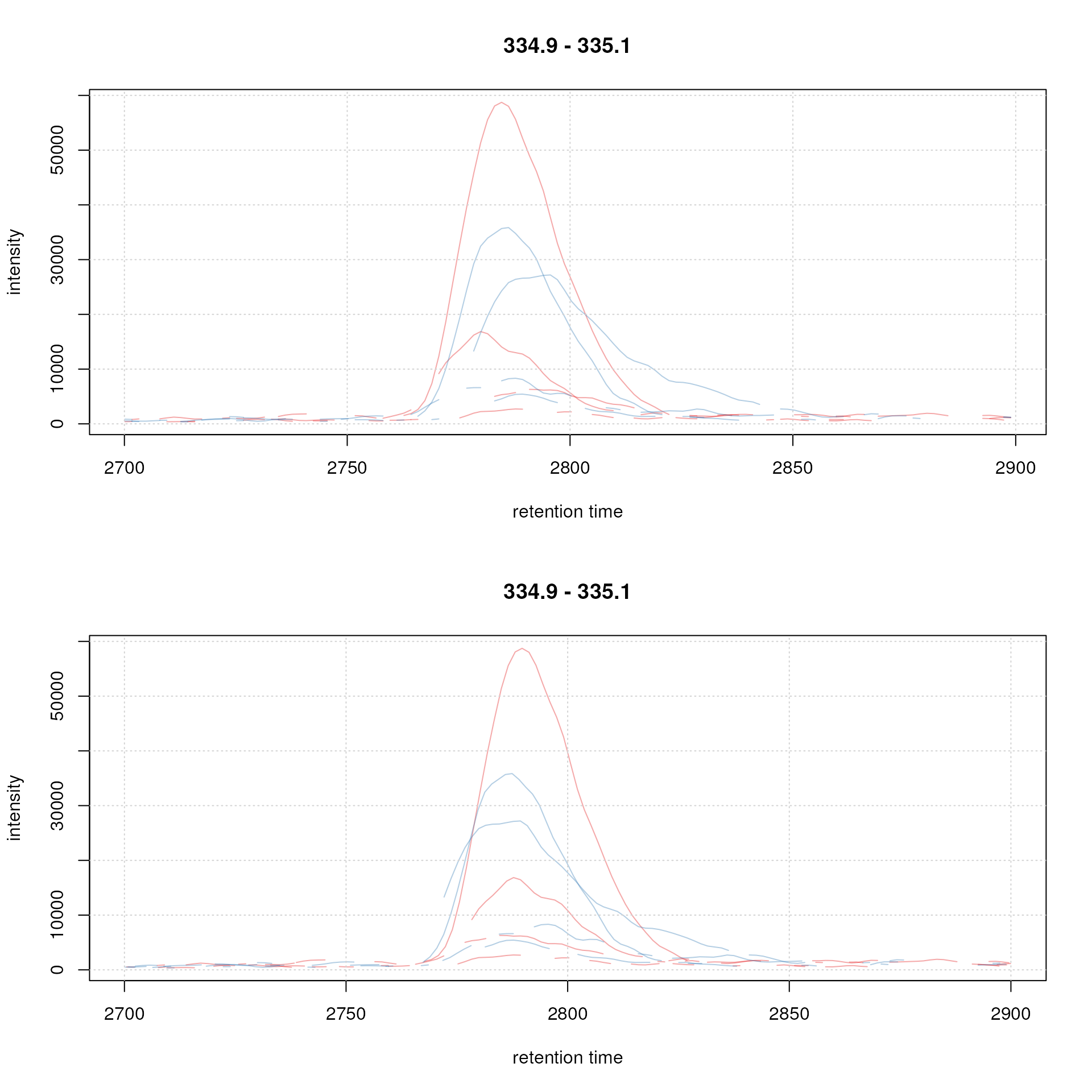
Example extracted ion chromatogram before (top) and after alignment (bottom).
Note: xcms result objects
(XcmsExperiment as well as XCMSnExp) contain
both the raw and the adjusted retention times for all spectra and subset
operation will in many cases drop adjusted retention times. Thus it
might sometimes be useful to immediately replace the
raw retention times in the data using the
applyAdjustedRtime() function.
Subset-based alignment
For some experiments it might be better to perform the alignment based on only a subset of the available samples, e.g. if pooled QC samples were injected at regular intervals or if the experiment contains blanks. All alignment methods in xcms support such a subset-based alignment in which retention time shifts are estimated on only a specified subset of samples followed by an alignment of the whole data set based on the aligned subset.
The subset of samples for such an alignment can be specified with the
parameter subset of the PeakGroupsParam or
ObiwarpParam object. Parameter subsetAdjust
allows to specify the method by which the left-out
samples will be adjusted. There are currently two options available:
subsetAdjust = "previous": adjust the retention times of a non-subset sample based on the alignment results of the previous subset sample (e.g. a QC sample). If samples are e.g. in the order A1, B1, B2, A2, B3, B4 with A representing QC samples and B study samples, usingsubset = c(1, 4)andsubsetAdjust = "previous"would result in all A samples to be aligned with each other and non-subset samples B1 and B2 being adjusted based on the alignment result of subset samples A1 and B3 and B4 on those of A2.subsetAdjust = "average": adjust retention times of non-subset samples based on an interpolation of the alignment results of the previous and subsequent subset sample. In the example above, B1 would be adjusted based on the average of adjusted retention times between subset (QC) samples A1 and A2. Since there is no subset sample after non-subset samples B3 and B4 these will be adjusted based on the alignment results of A2 alone. Note that a weighted average is used to calculate the adjusted retention time averages, which uses the inverse of the difference of the index of the non-subset sample to the subset samples as weights. Thus, if we have a setup like A1, B1, B2, A2 the adjusted retention times of A1 would get a larger weight than those of A2 in the adjustment of non-subset sample B1 causing it’s adjusted retention times to be closer to those of A1 than to A2. See below for examples.
Important: both cases require a meaningful/correct ordering of the samples within the object (i.e., samples should be ordered by injection index).
The examples below aim to illustrate the effect of these alignment
options. We assume samples 1, 4 and 7 in the faahKO data set to
be QC pool samples. We thus want to perform the alignment based on these
samples and subsequently adjust the retention times of the left-out
samples (2, 3, 5, 6 and 8) based on interpolation of the results from
the neighboring subset (QC) samples. After initial peak
grouping we perform the subset-based alignment with the peak
groups method by passing the indices of the QC samples with the
subset parameter to the PeakGroupsParam
function and set subsetAdjust = "average" to adjust the
study samples based on interpolation of the alignment results from
neighboring subset/QC samples.
Note that for any subset-alignment all parameters such as
minFraction are relative to the subset, not
the full experiment!
Below we first remove any previous alignment results with the
dropAdjustedRtime() function to allow a fresh alignment
using the subset-based option outlined above. In addition to removing
adjusted retention times for all spectra, this function will also
restore the original retention times for identified
chromatographic peaks.
faahko <- dropAdjustedRtime(faahko)

## Define the experimental layout
sampleData(faahko)$sample_type <- "study"
sampleData(faahko)$sample_type[c(1, 4, 7)] <- "QC"
For an alignment with the peak groups method an initial peak
grouping (correspondence) analysis is required, because the algorithm
estimates retention times shifts between samples using the retention
times of hook peaks (i.e. chromatographic peaks present in
most/all samples). Here we use the default settings for an peak
density method-based correspondence, but it is strongly advised to
adapt the parameters for each data set (details in the next section).
The definition of the sample groups (i.e. assignment of individual
samples to the sample groups in the experiment) is mandatory for the
PeakDensityParam. If there are no sample groups in the
experiment, sampleGroups should be set to a single value
for each file (e.g. rep(1, length(fileNames(faahko))).
## Initial peak grouping. Use sample_type as grouping variable
pdp_subs <- PeakDensityParam(sampleGroups = sampleData(faahko)$sample_type,
                             minFraction = 0.9)
faahko <- groupChromPeaks(faahko, param = pdp_subs)

## Define subset-alignment options and perform the alignment
pgp_subs <- PeakGroupsParam(
    minFraction = 0.85,
    subset = which(sampleData(faahko)$sample_type == "QC"),
    subsetAdjust = "average", span = 0.4)
faahko <- adjustRtime(faahko, param = pgp_subs)
Below we plot the results of the alignment highlighting the subset
samples in green. This nicely shows how the interpolation of the
subsetAdjust = "average" works: retention times of sample 2
are adjusted based on those from subset sample 1 and 4, giving however
more weight to the closer subset sample 1 which results in the adjusted
retention times of 2 being more similar to those of sample 1. Sample 3
on the other hand gets adjusted giving more weight to the second subset
sample (4).
clrs <- rep("#00000040", 8)
clrs[sampleData(faahko)$sample_type == "QC"] <- c("#00ce0080")
par(mfrow = c(2, 1), mar = c(4, 4.5, 1, 0.5))
plot(chromatogram(faahko, aggregationFun = "max", chromPeaks = "none"),
     col = clrs)
grid()
plotAdjustedRtime(faahko, col = clrs, peakGroupsPch = 1,
                  peakGroupsCol = "#00ce0040")
grid()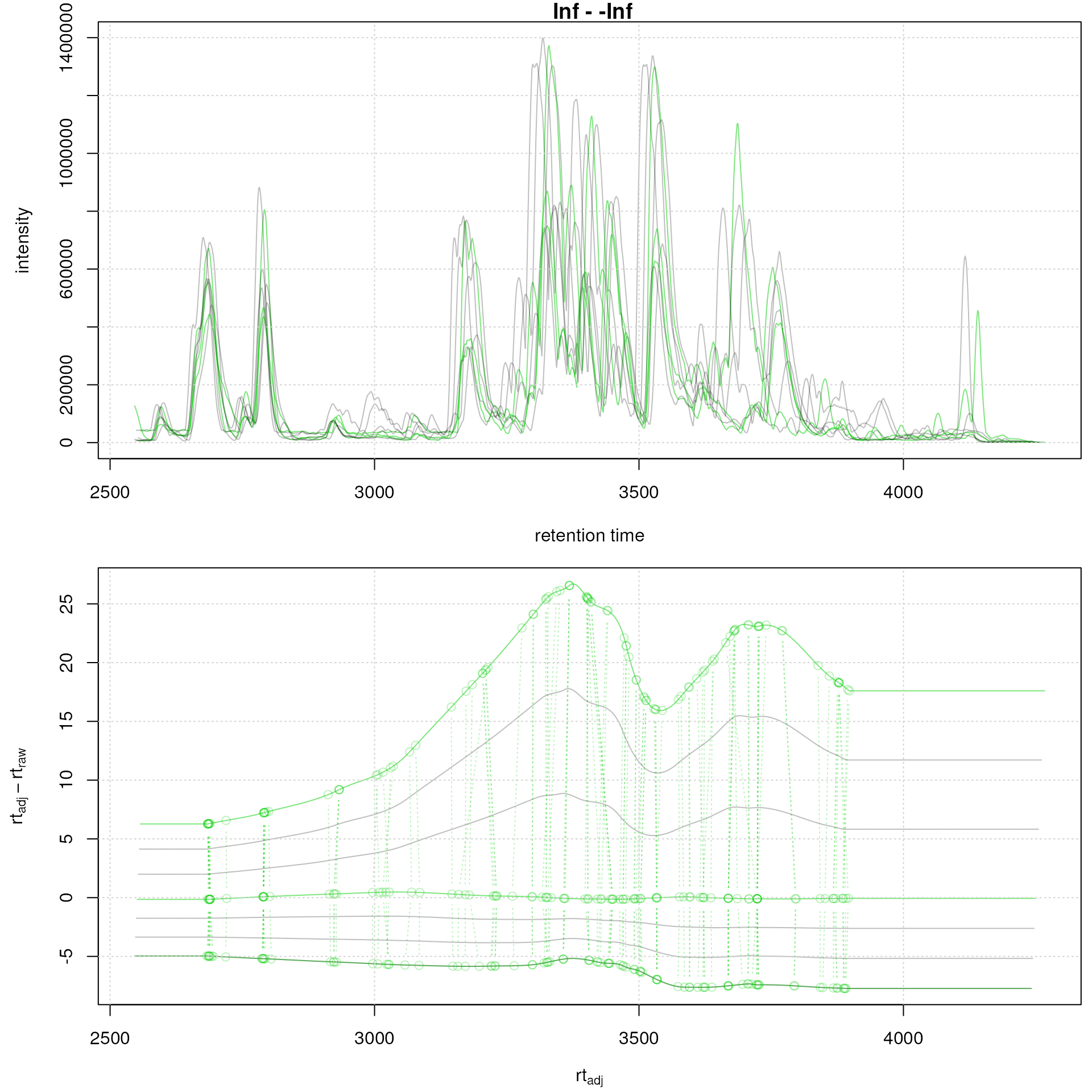
Subset-alignment results with option average. Difference between adjusted and raw retention times along the retention time axis. Samples on which the alignment models were estimated are shown in green, study samples in grey.
Option subsetAdjust = "previous" would adjust the
retention times of a non-subset sample based on a single subset sample
(the previous), which results in most cases in the adjusted retention
times of the non-subset sample being highly similar to those of the
subset sample which was used for adjustment.
Correspondence
Correspondence is usually the final step in LC-MS data preprocessing
in which data, presumably representing signal from the same originating
ions, is matched across samples. As a result, chromatographic peaks from
different samples with similar m/z and retention times get grouped into
LC-MS features. The function to perform the correspondence in
xcms is called groupChromPeaks() that again
supports different algorithms which can be selected and configured with
a specific parameter object (see ?groupChromPeaks for an
overview). For our example we will use the peak density method
[1] that, within small slices along the
m/z dimension, combines chromatographic peaks depending on the density
of these peaks along the retention time axis. To illustrate this, we
simulate below the peak grouping for an m/z slice containing
multiple chromatoghaphic peaks within each sample using the
plotChromPeakDensity() function and a
PeakDensityParam object with parameter
minFraction = 0.4 (features are only defined if in at least
40% of samples a chromatographic peak was present) - parameter
sampleGroups is used to define to which sample group each
sample belongs.
## Define the mz slice.
mzr <- c(305.05, 305.15)

## Extract and plot the chromatograms
chr_mzr <- chromatogram(faahko, mz = mzr)
## Define the parameters for the peak density method
pdp <- PeakDensityParam(sampleGroups = sampleData(faahko)$sample_group,
                        minFraction = 0.4, bw = 30)
plotChromPeakDensity(chr_mzr, col = sample_colors, param = pdp,
                     peakBg = sample_colors[chromPeaks(chr_mzr)[, "sample"]],
                     peakCol = sample_colors[chromPeaks(chr_mzr)[, "sample"]],
                     peakPch = 16)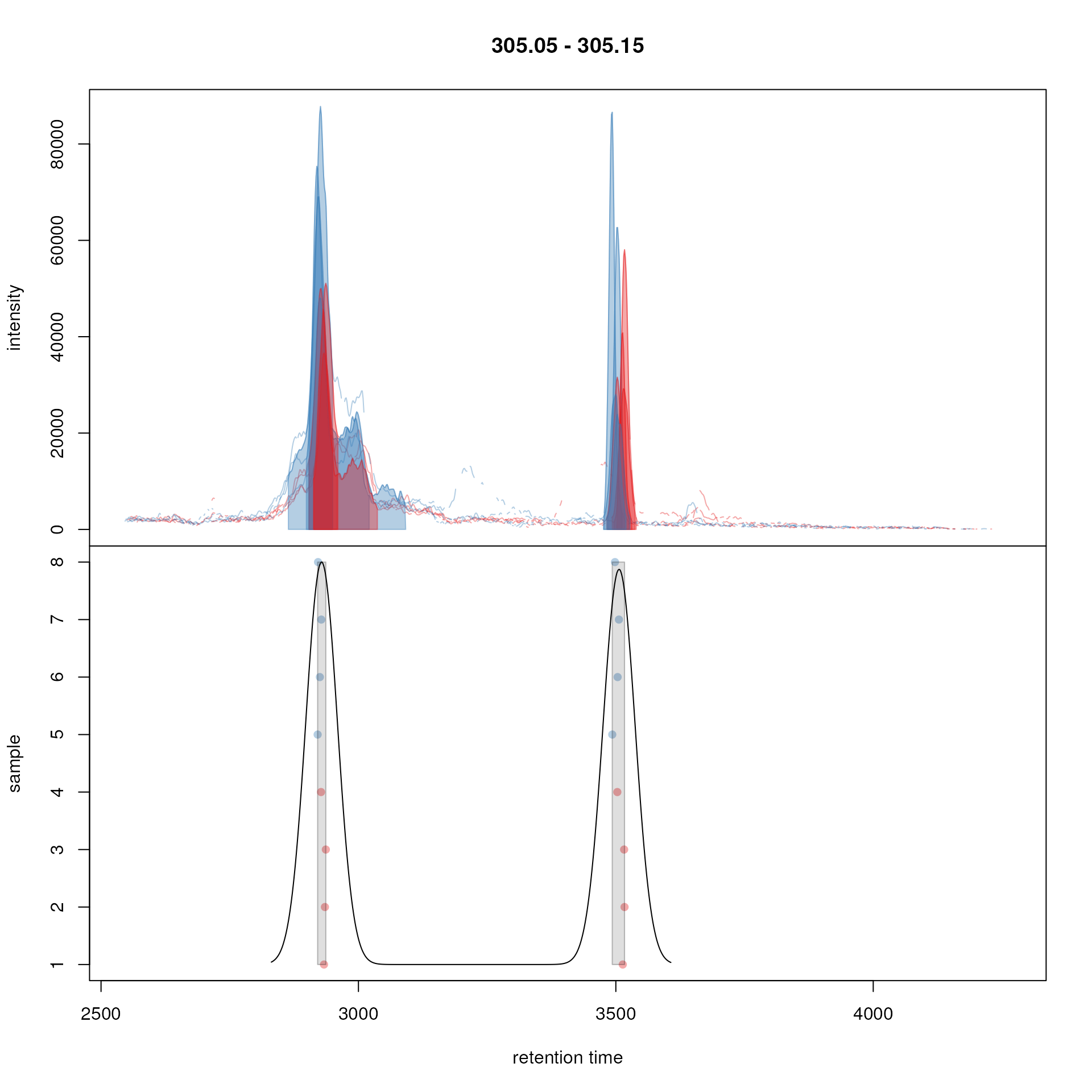
Example for peak density correspondence. Upper panel: chromatogram for an mz slice with multiple chromatographic peaks. lower panel: identified chromatographic peaks at their retention time (x-axis) and index within samples of the experiments (y-axis) for different values of the bw parameter. The black line represents the peak density estimate. Grouping of peaks (based on the provided settings) is indicated by grey rectangles.
The upper panel in the plot shows the extracted ion chromatogram for
each sample with the detected peaks highlighted. The retention times for
the individual chromatographic peaks in each sample (y-axis being the
index of the sample in the data set) are shown in the lower panel with
the solid black line representing the density estimate for the
distribution of detected peaks along the retention time. Parameter
bw defines the smoothness of this estimation. The
grey rectangles indicate which chromatographic peaks would be grouped
into a feature (each grey rectangle thus representing one feature). This
type of visualization is thus ideal to test, validate and optimize
correspondence settings on manually defined m/z slices before applying
them to the full data set. For the tested m/z slice the settings seemed
to be OK and we are thus applying them to the full data set below.
Especially the parameter bw will be very data set dependent
(or more specifically LC-dependent) and should be adapted to each data
set.
Another important parameter is binSize that defines the
size of the m/z slices (bins) within which peaks are being grouped. This
parameter thus defines the required similarity in m/z values for the
chromatographic peaks that are then assumed to represent signal from the
same (type of ion of a) compound and hence evaluated for grouping. By
default, a constant m/z bin size is used, but by changing parameter
ppm to a value larger than 0, m/z-relative bin sizes would
be used instead (i.e., the bin size will increase with the m/z value
hence better representing the measurement error/precision of some MS
instruments). The bin sizes (and subsequently the m/z width of the
defined features) would then reach a maximal value of
binSize plus ppm parts-per-million of the
largest m/z value of any chromatographic peak in the data set.
See also the xcms tutorial for more examples and details.
## Perform the correspondence using fixed m/z bin sizes.
pdp <- PeakDensityParam(sampleGroups = sampleData(faahko)$sample_group,
                        minFraction = 0.4, bw = 30)
faahko <- groupChromPeaks(faahko, param = pdp)
As an alternative we perform the correspondence using m/z relative bin sizes.
## Drop feature definitions and re-perform the correspondence
## using m/z-relative bin sizes.
faahko_ppm <- groupChromPeaks(
    dropFeatureDefinitions(faahko),
    PeakDensityParam(sampleGroups = sampleData(faahko)$sample_group,
                     minFraction = 0.4, bw = 30, ppm = 10))
The results will be mostly similar, except for the higher m/z range (in which larger m/z bins will be used). Below we plot the m/z range for features against their median m/z. For the present data set (acquired with a triple quad instrument) no clear difference can be seen for the two approaches hence we proceed the analysis with the fixed bin size setting. A stronger relationship would be expected for example for data measured on TOF instruments.
## Calculate m/z width of features
mzw <- featureDefinitions(faahko)$mzmax - featureDefinitions(faahko)$mzmin
mzw_ppm <- featureDefinitions(faahko_ppm)$mzmax -
                                        featureDefinitions(faahko_ppm)$mzmin
plot(featureDefinitions(faahko_ppm)$mzmed, mzw_ppm,
     xlab = "m/z", ylab = "m/z width", pch = 21,
     col = "#0000ff20", bg = "#0000ff10")
points(featureDefinitions(faahko)$mzmed, mzw, pch = 21,
     col = "#ff000020", bg = "#ff000010")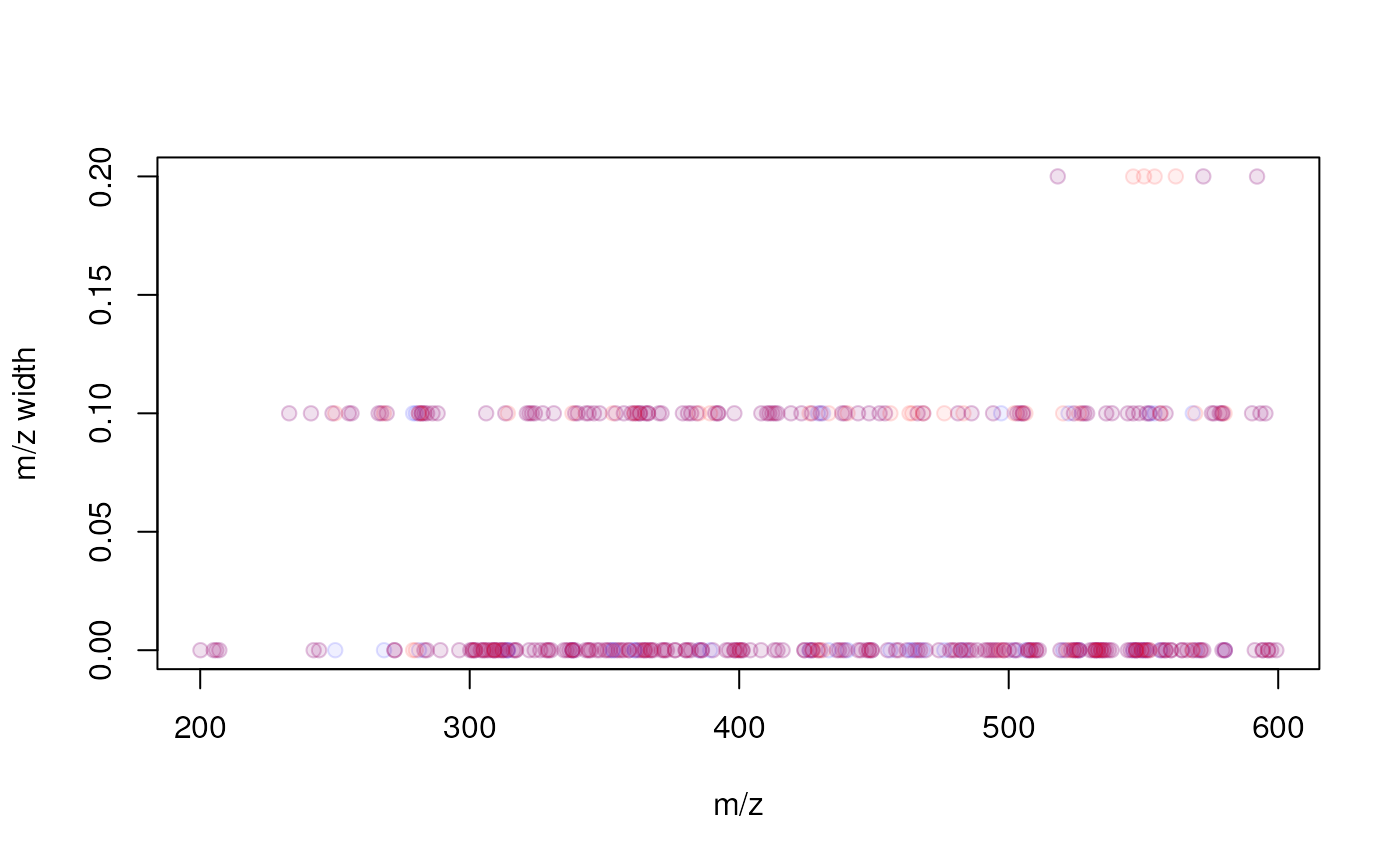
Relationship between a feature’s m/z and the m/z width (max - min m/z) of the feature. Red points represent the results with the fixed m/z bin size, blue with the m/z-relative bin size.
Results from the correspondence analysis can be accessed with the
featureDefinitions() and featureValues()
function. The former returns a data frame with general information on
each of the defined features, with each row being one feature and
columns providing information on the median m/z and retention time as
well as the indices of the chromatographic peaks assigned to the feature
in column "peakidx". Below we show the information on the
first 6 features.
featureDefinitions(faahko) |> head()## mzmed mzmin mzmax rtmed rtmin rtmax npeaks KO WT peakidx
## FT001 200.1 200.1 200.1 2902.634 2882.603 2922.664 2 2 0 458, 1161
## FT002 205.0 205.0 205.0 2789.901 2782.955 2796.531 8 4 4 44, 443,....
## FT003 206.0 206.0 206.0 2789.405 2781.389 2794.219 7 3 4 29, 430,....
## FT004 207.1 207.1 207.1 2718.560 2714.047 2727.347 7 4 3 16, 420,....
## FT005 233.0 233.0 233.1 3023.579 3015.145 3043.959 7 3 4 69, 959,....
## FT006 241.1 241.1 241.2 3683.299 3661.586 3695.886 8 3 4 276, 284....
## ms_level
## FT001 1
## FT002 1
## FT003 1
## FT004 1
## FT005 1
## FT006 1The featureValues() function returns a
matrix with rows being features and columns samples. The
content of this matrix can be defined using the value
argument which can be any column name in the chromPeaks()
matrix. With the default value = "into" a matrix with the
integrated signal of the peaks corresponding to a feature in a sample
are returned. This is then generally used as the intensity matrix for
downstream analysis. Below we extract the intensities for the first 6
features.
featureValues(faahko, value = "into") |> head()## ko15.CDF ko16.CDF ko21.CDF ko22.CDF wt15.CDF wt16.CDF wt21.CDF
## FT001 NA 506848.9 NA 169955.6 NA NA NA
## FT002 1924712.0 1757151.0 1383416.7 1180288.2 2129885.1 1634342.0 1623589.2
## FT003 213659.3 289500.7 NA 178285.7 253825.6 241844.4 240606.0
## FT004 349011.5 451863.7 343897.8 208002.8 364609.8 360908.9 NA
## FT005 286221.4 NA 164009.0 149097.6 255697.7 311296.8 366441.5
## FT006 1160580.5 NA 380970.3 588986.4 1286883.0 1739516.6 639755.3
## wt22.CDF
## FT001 NA
## FT002 1354004.9
## FT003 185399.5
## FT004 221937.5
## FT005 271128.0
## FT006 508546.4As we can see we have several missing values in this feature matrix. Missing values are reported if in one sample no chromatographic peak was detected in the m/z - rt region of the feature. This does however not necessarily mean that there is no signal for that specific ion in that sample. The chromatographic peak detection algorithm could also just have failed to identify any peak in that region, e.g. because the signal was too noisy or too low. Thus it is advisable to perform, after correspondence, also a gap-filling (see next section).
The performance of peak detection, alignment and correspondence
should always be evaluated by inspecting extracted ion chromatograms
e.g. of known compounds, internal standards or identified features in
general. The featureChromatograms() function allows to
extract chromatograms for each feature present in
featureDefinitions(). The returned
MChromatograms object contains an ion chromatogram for each
feature (each row containing the data for one feature) and sample (each
column representing containing data for one sample). Parameter
features allows to define specific features for which the
EIC should be returned. These can be specified with their index or their
ID (i.e. their row name in the featureDefinitions() data
frame. If features is not defined, EICs are returned for
all features in a data set, which can take also a
considerable amount of time. Below we extract the chromatograms for the
first 4 features.
feature_chroms <- featureChromatograms(faahko, features = 1:4)

feature_chroms
## XChromatograms with 4 rows and 8 columns
## ko15.CDF ko16.CDF ko21.CDF ko22.CDF
## <XChromatogram> <XChromatogram> <XChromatogram> <XChromatogram>
## [1,] peaks: 0 peaks: 1 peaks: 0 peaks: 1
## [2,] peaks: 1 peaks: 1 peaks: 1 peaks: 1
## [3,] peaks: 1 peaks: 1 peaks: 0 peaks: 1
## [4,] peaks: 1 peaks: 1 peaks: 1 peaks: 1
## wt15.CDF wt16.CDF wt21.CDF wt22.CDF
## <XChromatogram> <XChromatogram> <XChromatogram> <XChromatogram>
## [1,] peaks: 0 peaks: 0 peaks: 0 peaks: 0
## [2,] peaks: 1 peaks: 1 peaks: 1 peaks: 1
## [3,] peaks: 1 peaks: 1 peaks: 1 peaks: 1
## [4,] peaks: 1 peaks: 1 peaks: 0 peaks: 1
## phenoData with 4 variables
## featureData with 4 variables
## - - - xcms preprocessing - - -
## Chromatographic peak detection:
## method: centWave
## Correspondence:
## method: chromatographic peak density
## 4 feature(s) identified.And plot the extracted ion chromatograms. We again use the group color for each identified peak to fill the area.
plot(feature_chroms, col = sample_colors,
     peakBg = sample_colors[chromPeaks(feature_chroms)[, "sample"]])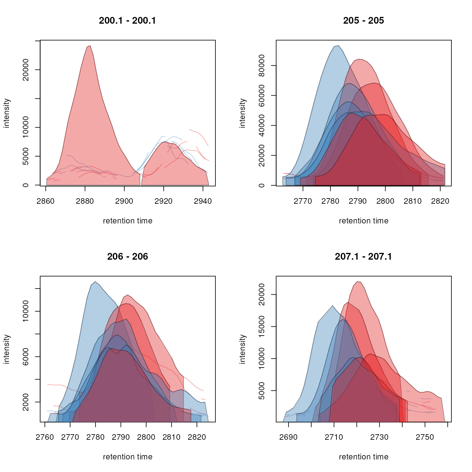
Extracted ion chromatograms for features 1 to 4.
To access the EICs of the second feature we can simply subset the
feature_chroms object.
eic_2 <- feature_chroms[2, ]
chromPeaks(eic_2)
## mz mzmin mzmax rt rtmin rtmax into intb maxo sn
## CP0048 205 205 205 2791.873 2771.300 2815.623 1924712 1850331 84280 64
## CP0495 205 205 205 2795.796 2773.702 2821.043 1757151 1711473 68384 69
## CP1033 205 205 205 2796.531 2774.506 2821.697 1383417 1334570 47384 54
## CP1255 205 205 205 2789.405 2769.019 2812.924 1180288 1126958 48336 32
## CP1535 205 205 205 2782.955 2762.596 2806.444 2129885 2054677 93312 44
## CP1967 205 205 205 2787.464 2767.135 2812.486 1634342 1566379 67984 53
## CP2350 205 205 205 2790.396 2763.847 2821.630 1623589 1531573 49208 28
## CP2601 205 205 205 2787.273 2766.970 2812.261 1354005 1299188 55712 35
## sample row column
## CP0048 1 1 1
## CP0495 2 1 2
## CP1033 3 1 3
## CP1255 4 1 4
## CP1535 5 1 5
## CP1967 6 1 6
## CP2350 7 1 7
## CP2601 8 1 8Gap filling
Missing values in LC-MS data are in many cases the result of the
chromatographic peak detection algorithm failing to identify peaks
(because of noisy or low intensity signal). The aim of the gap filling
step is to reduce the number of such missing values by integrating
signals from the original data files for samples in which no
chromatographic peak was found from the m/z - rt region where signal
from the ion is expected. Gap filling can be performed in xcms
with the fillChromPeaks() function and a parameter object
selecting and configuring the gap filling algorithm. The method of
choice is ChromPeakAreaParam that integrates the signal (in
samples in which no chromatographic peak was found for a feature) in the
m/z - rt region that is defined based on the m/z and retention time
ranges of all detected chromatographic peaks of that specific feature.
The lower m/z limit of the area is defined as the lower quartile (25%
quantile) of the "mzmin" values of all peaks of the
feature, the upper m/z value as the upper quartile (75% quantile) of the
"mzmax" values, the lower rt value as the lower quartile
(25% quantile) of the "rtmin" and the upper rt value as the
upper quartile (75% quantile) of the "rtmax" values. An
additional parameter minMzWidthPpm allows to define a
minimal guaranteed m/z width (expressed in ppm of the features’
m/z value) of the area to integrate signal from.
Below we perform this gap filling on our test data and extract the
feature values for the first 6 features after gap filling. An
NA is reported if no signal is measured at all for a
specific sample.
faahko <- fillChromPeaks(faahko, param = ChromPeakAreaParam())

featureValues(faahko, value = "into") |> head()
## ko15.CDF ko16.CDF ko21.CDF ko22.CDF wt15.CDF wt16.CDF wt21.CDF
## FT001 135162.4 506848.9 111657.3 169955.6 209929.4 141607.9 226853.7
## FT002 1924712.0 1757151.0 1383416.7 1180288.2 2129885.1 1634342.0 1623589.2
## FT003 213659.3 289500.7 164380.7 178285.7 253825.6 241844.4 240606.0
## FT004 349011.5 451863.7 343897.8 208002.8 364609.8 360908.9 226234.4
## FT005 286221.4 285857.6 164009.0 149097.6 255697.7 311296.8 366441.5
## FT006 1160580.5 1102832.6 380970.3 588986.4 1286883.0 1739516.6 639755.3
## wt22.CDF
## FT001 138341.2
## FT002 1354004.9
## FT003 185399.5
## FT004 221937.5
## FT005 271128.0
## FT006 508546.4Final result
While we can continue using the xcms result set for further
analysis (e.g. also for feature grouping with the MsFeatures
package; see the LC-MS feature grouping vignette for details) we could
also extract all results as a SummarizedExperiment object.
This is the standard data container for Bioconductor defined in
the SummarizedExperiment
package and integration with other Bioconductor packages might thus be
easier using that type of object. Below we use the
quantify() function to extract the xcms
preprocessing results as such a SummarizedExperiment
object. Internally, the featureValues() function is used to
generate the feature value matrix. We can pass any parameters from that
function to the quantify() call. Below we use
value = "into" and method = "sum" to report
the integrated peak signal as intensity and to sum these values in
samples in which more than one chromatographic peak was assigned to a
feature (for that option it is important to run
refineChromPeaks() like described above to merge
overlapping peaks in each sample).
## Loading required package: MatrixGenerics## Loading required package: matrixStats##
## Attaching package: 'MatrixGenerics'## The following objects are masked from 'package:matrixStats':
##
## colAlls, colAnyNAs, colAnys, colAvgsPerRowSet, colCollapse,
## colCounts, colCummaxs, colCummins, colCumprods, colCumsums,
## colDiffs, colIQRDiffs, colIQRs, colLogSumExps, colMadDiffs,
## colMads, colMaxs, colMeans2, colMedians, colMins, colOrderStats,
## colProds, colQuantiles, colRanges, colRanks, colSdDiffs, colSds,
## colSums2, colTabulates, colVarDiffs, colVars, colWeightedMads,
## colWeightedMeans, colWeightedMedians, colWeightedSds,
## colWeightedVars, rowAlls, rowAnyNAs, rowAnys, rowAvgsPerColSet,
## rowCollapse, rowCounts, rowCummaxs, rowCummins, rowCumprods,
## rowCumsums, rowDiffs, rowIQRDiffs, rowIQRs, rowLogSumExps,
## rowMadDiffs, rowMads, rowMaxs, rowMeans2, rowMedians, rowMins,
## rowOrderStats, rowProds, rowQuantiles, rowRanges, rowRanks,
## rowSdDiffs, rowSds, rowSums2, rowTabulates, rowVarDiffs, rowVars,
## rowWeightedMads, rowWeightedMeans, rowWeightedMedians,
## rowWeightedSds, rowWeightedVars## Loading required package: GenomicRanges## Loading required package: stats4## Loading required package: BiocGenerics## Loading required package: generics##
## Attaching package: 'generics'## The following objects are masked from 'package:base':
##
## as.difftime, as.factor, as.ordered, intersect, is.element, setdiff,
## setequal, union##
## Attaching package: 'BiocGenerics'## The following objects are masked from 'package:stats':
##
## IQR, mad, sd, var, xtabs## The following objects are masked from 'package:base':
##
## anyDuplicated, aperm, append, as.data.frame, basename, cbind,
## colnames, dirname, do.call, duplicated, eval, evalq, Filter, Find,
## get, grep, grepl, is.unsorted, lapply, Map, mapply, match, mget,
## order, paste, pmax, pmax.int, pmin, pmin.int, Position, rank,
## rbind, Reduce, rownames, sapply, saveRDS, table, tapply, unique,
## unsplit, which.max, which.min## Loading required package: S4Vectors##
## Attaching package: 'S4Vectors'## The following object is masked from 'package:utils':
##
## findMatches## The following objects are masked from 'package:base':
##
## expand.grid, I, unname## Loading required package: IRanges## Loading required package: Seqinfo## Loading required package: Biobase## Welcome to Bioconductor
##
## Vignettes contain introductory material; view with
## 'browseVignettes()'. To cite Bioconductor, see
## 'citation("Biobase")', and for packages 'citation("pkgname")'.##
## Attaching package: 'Biobase'## The following object is masked from 'package:MatrixGenerics':
##
## rowMedians## The following objects are masked from 'package:matrixStats':
##
## anyMissing, rowMedians
res <- quantify(faahko, value = "into", method = "sum")
res
## class: SummarizedExperiment
## dim: 351 8
## metadata(6): '' '' ... '' ''
## assays(1): raw
## rownames(351): FT001 FT002 ... FT350 FT351
## rowData names(10): mzmed mzmin ... WT ms_level
## colnames(8): ko15.CDF ko16.CDF ... wt21.CDF wt22.CDF
## colData names(4): sample_name sample_group spectraOrigin sample_typeThe information from featureDefinitions() is now stored
in the rowData() of this object. The rowData()
provides annotations and information for each row in
the SummarizedExperiment (which in our case are the
features).
rowData(res)## DataFrame with 351 rows and 10 columns
## mzmed mzmin mzmax rtmed rtmin rtmax npeaks
## <numeric> <numeric> <numeric> <numeric> <numeric> <numeric> <numeric>
## FT001 200.1 200.1 200.1 2902.63 2882.60 2922.66 2
## FT002 205.0 205.0 205.0 2789.90 2782.95 2796.53 8
## FT003 206.0 206.0 206.0 2789.40 2781.39 2794.22 7
## FT004 207.1 207.1 207.1 2718.56 2714.05 2727.35 7
## FT005 233.0 233.0 233.1 3023.58 3015.14 3043.96 7
## ... ... ... ... ... ... ... ...
## FT347 595.25 595.2 595.3 3010.60 2992.76 3014.37 6
## FT348 596.20 596.2 596.2 2997.78 2992.76 3002.79 2
## FT349 596.30 596.3 596.3 3819.83 3811.52 3836.39 4
## FT350 597.40 597.4 597.4 3820.88 3817.76 3826.13 3
## FT351 599.30 599.3 599.3 4071.41 4044.94 4125.32 3
## KO WT ms_level
## <numeric> <numeric> <integer>
## FT001 2 0 1
## FT002 4 4 1
## FT003 3 4 1
## FT004 4 3 1
## FT005 3 4 1
## ... ... ... ...
## FT347 2 3 1
## FT348 0 2 1
## FT349 2 2 1
## FT350 1 2 1
## FT351 1 2 1Annotations for columns (in our case
samples) are stored as colData(). In this
data frame each row contains annotations for one sample (and hence one
column in the feature values matrix).
colData(res)## DataFrame with 8 rows and 4 columns
## sample_name sample_group spectraOrigin sample_type
## <character> <character> <character> <character>
## ko15.CDF ko15 KO /__w/_temp... QC
## ko16.CDF ko16 KO /__w/_temp... study
## ko21.CDF ko21 KO /__w/_temp... study
## ko22.CDF ko22 KO /__w/_temp... QC
## wt15.CDF wt15 WT /__w/_temp... study
## wt16.CDF wt16 WT /__w/_temp... study
## wt21.CDF wt21 WT /__w/_temp... QC
## wt22.CDF wt22 WT /__w/_temp... studyFinally, the feature matrix is stored as an assay within the
object. Note that a SummarizedExperiment can have multiple
assays which have to be numeric matrices with the number of rows and
columns matching the number of features and samples, respectively. Below
we list the names of the available assays.
assayNames(res)## [1] "raw"And we can access the actual data using the assay()
function, optionally also providing the name of the assay we want to
access. Below we show the first 6 lines of that matrix.
##        ko15.CDF  ko16.CDF  ko21.CDF  ko22.CDF  wt15.CDF  wt16.CDF  wt21.CDF
## FT001  135162.4  506848.9  111657.3  169955.6  209929.4  141607.9  226853.7
## FT002 1924712.0 1757151.0 1383416.7 1180288.2 2129885.1 1634342.0 1623589.2
## FT003  213659.3  289500.7  164380.7  178285.7  253825.6  241844.4  240606.0
## FT004  349011.5  451863.7  343897.8  208002.8  364609.8  360908.9  226234.4
## FT005  286221.4  285857.6  164009.0  149097.6  255697.7  311296.8  366441.5
## FT006 1923307.8 1102832.6  380970.3  588986.4 1286883.0 1739516.6  639755.3
##        wt22.CDF
## FT001  138341.2
## FT002 1354004.9
## FT003  185399.5
## FT004  221937.5
## FT005  271128.0
## FT006  508546.4
Since a SummarizedExperiment supports multiple assays,
we in addition add also the feature value matrix
without filled-in values (i.e. feature intensities that
were added by the gap filling step).
assays(res)$raw_nofill <- featureValues(faahko, filled = FALSE, method = "sum")With that we have now two assays in our result object.
assayNames(res)## [1] "raw" "raw_nofill"And we can extract the feature values without gap-filling:
##        ko15.CDF  ko16.CDF  ko21.CDF  ko22.CDF  wt15.CDF  wt16.CDF  wt21.CDF
## FT001        NA  506848.9        NA  169955.6        NA        NA        NA
## FT002 1924712.0 1757151.0 1383416.7 1180288.2 2129885.1 1634342.0 1623589.2
## FT003  213659.3  289500.7        NA  178285.7  253825.6  241844.4  240606.0
## FT004  349011.5  451863.7  343897.8  208002.8  364609.8  360908.9        NA
## FT005  286221.4        NA  164009.0  149097.6  255697.7  311296.8  366441.5
## FT006 1923307.8        NA  380970.3  588986.4 1286883.0 1739516.6  639755.3
##        wt22.CDF
## FT001        NA
## FT002 1354004.9
## FT003  185399.5
## FT004  221937.5
## FT005  271128.0
## FT006  508546.4
Finally, a history of the full processing with xcms is
available as metadata in the
SummarizedExperiment.
metadata(res)## [[1]]
## Object of class "XProcessHistory"
##  type: Peak detection
##  date: Wed Apr 22 11:07:44 2026
##  info:
##  fileIndex: 1,2,3,4,5,6,7,8
##  Parameter class: CentWaveParam
##  MS level(s) 1
##
## [[2]]
## Object of class "XProcessHistory"
## type: Peak refinement
## date: Wed Apr 22 11:07:49 2026
## info:
## fileIndex: 1,2,3,4,5,6,7,8
## Parameter class: MergeNeighboringPeaksParam
## MS level(s) 1
##
## [[3]]
## Object of class "XProcessHistory"
## type: Peak grouping
## date: Wed Apr 22 11:08:01 2026
## info:
## fileIndex: 1,2,3,4,5,6,7,8
## Parameter class: PeakDensityParam
## MS level(s) 1
##
## [[4]]
## Object of class "XProcessHistory"
## type: Retention time correction
## date: Wed Apr 22 11:08:02 2026
## info:
## fileIndex: 1,2,3,4,5,6,7,8
## Parameter class: PeakGroupsParam
## MS level(s) 1
##
## [[5]]
## Object of class "XProcessHistory"
## type: Peak grouping
## date: Wed Apr 22 11:08:06 2026
## info:
## fileIndex: 1,2,3,4,5,6,7,8
## Parameter class: PeakDensityParam
## MS level(s) 1
##
## [[6]]
## Object of class "XProcessHistory"
## type: Missing peak filling
## date: Wed Apr 22 11:08:10 2026
## info:
## fileIndex: 1,2,3,4,5,6,7,8
## Parameter class: ChromPeakAreaParam
## MS level(s) 1This same information can also be extracted from the xcms
result object using the processHistory() function. Below we
extract the information for the first processing step.
processHistory(faahko)[[1]]## Object of class "XProcessHistory"
## type: Peak detection
## date: Wed Apr 22 11:07:44 2026
## info:
## fileIndex: 1,2,3,4,5,6,7,8
## Parameter class: CentWaveParam
## MS level(s) 1These processing steps contain also the individual parameter objects used for the analysis, hence allowing to exactly reproduce the analysis.
processHistory(faahko)[[1]] |> processParam()## Object of class: CentWaveParam
## Parameters:
## - ppm: [1] 25
## - peakwidth: [1] 20 80
## - snthresh: [1] 10
## - prefilter: [1] 6 5000
## - mzCenterFun: [1] "wMean"
## - integrate: [1] 1
## - mzdiff: [1] -0.001
## - fitgauss: [1] FALSE
## - noise: [1] 5000
## - verboseColumns: [1] FALSE
## - roiList: list()
## - firstBaselineCheck: [1] TRUE
## - roiScales: numeric(0)
## - extendLengthMSW: [1] FALSE
## - verboseBetaColumns: [1] FALSEAt last we perform also a principal component analysis to evaluate the grouping of the samples in this experiment. Note that we did not perform any data normalization hence the grouping might (and will) also be influenced by technical biases.
## Extract the features and log2 transform them
ft_ints <- log2(assay(res, "raw"))

## Perform the PCA omitting all features with an NA in any of the
## samples. Also, the intensities are mean centered.
pc <- prcomp(t(na.omit(ft_ints)), center = TRUE)

## Plot the PCA
pcSummary <- summary(pc)
plot(pc$x[, 1], pc$x[,2], pch = 21, main = "",
     xlab = paste0("PC1: ", format(pcSummary$importance[2, 1] * 100,
                                   digits = 3), " % variance"),
     ylab = paste0("PC2: ", format(pcSummary$importance[2, 2] * 100,
                                   digits = 3), " % variance"),
     col = "darkgrey", bg = sample_colors, cex = 2)
grid()
text(pc$x[, 1], pc$x[,2], labels = res$sample_name, col = "darkgrey",
     pos = 3, cex = 2)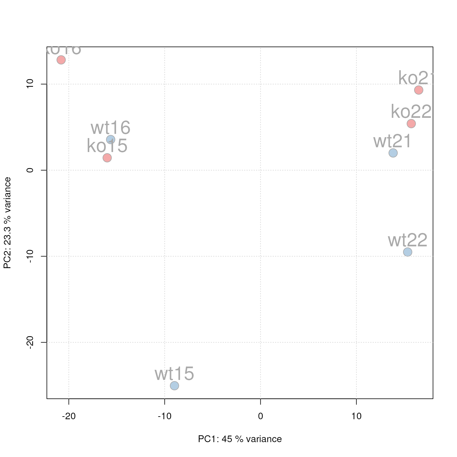
PCA for the faahKO data set, un-normalized intensities.
We can see the expected separation between the KO and WT samples on PC2. On PC1 samples separate based on their ID, samples with an ID <= 18 from samples with an ID > 18. This separation might be caused by a technical bias (e.g. measurements performed on different days/weeks) or due to biological properties of the mice analyzed (sex, age, litter mates etc).
Further data processing and analysis
Quality-based filtering of features
When dealing with metabolomics results, it is often necessary to
filter features based on certain criteria. These criteria are typically
derived from statistical formulas applied to full rows of data, where
each row represents a feature. The filterFeatures()
function provides a robust solution for filtering features based on
these conventional quality assessment criteria. It supports multiple
types of filtering, allowing users to tailor the filtering process to
their specific needs, all controlled by the filter
argument. This function and its implementations are applicable to both
XcmsExperiment results objects and
SummarizedExperiment objects.
We will demonstrate how to use the filterFeatures()
function to perform quality assessment and filtering on both the
faahko and res variables defined above. The
filter argument can accommodate various types of input,
each determining the specific type of quality assessment and filtering
to be performed.
The PercentMissingFilter allows to filter features based
on the percentage of missing values for each feature. This function
takes as an input the parameter f which is supposed to be a
vector of length equal to the length of the object (i.e. number of
samples) with the sample type for each. The function then computes the
percentage of missing values per sample groups and filters features
based on this. Features with a percent of missing values larger than the
threshold in all sample groups will be removed. Another option is to
base this quality assessment and filtering only on QC samples.
Both examples are shown below:
# To set up parameter `f` to filter only based on QC samples
f <- sampleData(faahko)$sample_type
f[f != "QC"] <- NA

# To set up parameter `f` to filter per sample type excluding QC samples
f <- sampleData(faahko)$sample_type
f[f == "QC"] <- NA

missing_filter <- PercentMissingFilter(threshold = 30, f = f)
# Apply the filter to faakho object
filtered_faahko <- filterFeatures(object = faahko, filter = missing_filter)
## 3 features were removed
# Apply the filter to res object
missing_filter <- PercentMissingFilter(threshold = 30, f = f)
filtered_res <- filterFeatures(object = res, filter = missing_filter)
## 3 features were removedHere, no feature was removed, meaning that all the features had less
than 30% of NA values in at least one of the sample
type.
Although not directly relevant to this experiment, the
BlankFlag filter can be used to flag features based on the
intensity relationship between blank and QC samples. More information
can be found in the documentation of the filter, i.e. using
?filterFeatures or ?BlankFlag.
The RsdFilter enable users to filter features based on
their relative standard deviation (coefficient of variation) for a
specified threshold. It is recommended to base the
computation on quality control (QC) samples, as demonstrated below:
# Set up parameters for RsdFilter
rsd_filter <- RsdFilter(
    threshold = 0.3,
    qcIndex = sampleData(filtered_faahko)$sample_type == "QC")

# Apply the filter to faakho object
filtered_faahko <- filterFeatures(object = filtered_faahko, filter = rsd_filter)
## 252 features were removed
# Now apply the same strategy to the res object
rsd_filter <- RsdFilter(
    threshold = 0.3, qcIndex = filtered_res$sample_type == "QC")
filtered_res <- filterFeatures(
    object = filtered_res, filter = rsd_filter, assay = "raw")
## 257 features were removedAll features with an RSD (CV) strictly larger than 0.3 in QC samples were thus removed from the data set.
The DratioFilter can be used to filter features based on
the D-ratio or dispersion ratio, which compares the standard
deviation in QC samples to that in study samples.
# Set up parameters for DratioFilter
dratio_filter <- DratioFilter(
    threshold = 0.5,
    qcIndex = sampleData(filtered_faahko)$sample_type == "QC",
    studyIndex = sampleData(filtered_faahko)$sample_type == "study")

# Apply the filter to faahko object
filtered_faakho <- filterFeatures(object = filtered_faahko,
                                  filter = dratio_filter)
## 38 features were removed
# Now same but for the res object
dratio_filter <- DratioFilter(
    threshold = 0.5,
    qcIndex = filtered_res$sample_type == "QC",
    studyIndex = filtered_res$sample_type == "study")

filtered_res <- filterFeatures(object = filtered_res,
                               filter = dratio_filter)
## 38 features were removedAll features with an D-ratio strictly larger than 0.5 were thus removed from the data set.
Alignment to an external reference dataset
In certain experiments, aligning two different datasets is necessary.
This can involve comparing runs of the same samples conducted across
different laboratories or runs with MS2 recorded after the initial MS1
run. Across laboratories and over time, the same samples may result in
variation in retention time, especially because the LC system can be
quite unstable. In these cases, an alignment step using the
adjustRtime() function with the LamaParam
parameter can allow the user to perform this type of alignment. We will
go through this step by step below.
Let’s load an already analyzed dataset ref and our
previous dataset before alignment, which will be tst. We
will first restrict their retention time range to be the same for both
dataset.
ref <- loadXcmsData("xmse")
tst <- loadXcmsData("faahko_sub2")
Now, we will attempt to align these two samples with the previous
dataset. The first step is to extract landmark features (referred to as
lamas). To achieve this, we will identify the features present
in every QC sample of the ref dataset. To do so, we will
categorize (using factor()) our data by
sample_type and only retain the QC samples. This variable
will be utilized to filter the features using the
PercentMissingFilter parameter within the
filterFeatures() function (see section above for more
information on this method)
f <- sampleData(ref)$sample_type
f[f != "QC"] <- NA
ref <- filterFeatures(ref, PercentMissingFilter(threshold = 0, f = f))
## 4 features were removed
ref_mz_rt <- featureDefinitions(ref)[, c("mzmed","rtmed")]
head(ref_mz_rt)
## mzmed rtmed
## FT001 200.1 2902.634
## FT002 205.0 2789.901
## FT003 206.0 2789.405
## FT004 207.1 2718.560
## FT005 233.0 3023.579
## FT006 241.1 3683.299
nrow(ref_mz_rt)## [1] 347This is what the lamas input should look like for alignment. In terms of how this method works, the alignment algorithm matches chromatographic peaks from the experimental data to the lamas, fitting a model based on this match to adjust their retention times and minimize differences between the two datasets.
Now we can define our param object
LamaParama to prepare for the alignment. Parameters such as
tolerance, toleranceRt, and ppm
relate to the matching between chromatographic peaks and lamas.
Other parameters are related to the type of fitting generated between
these data points. More details on each parameter and the overall method
can be found by searching ?adjustRtime. Below is an example
using default parameters.
param <- LamaParama(lamas = ref_mz_rt, method = "loess", span = 0.5,
                    outlierTolerance = 3, zeroWeight = 10, ppm = 20,
                    tolerance = 0, toleranceRt = 20, bs = "tp")

#' input into `adjustRtime()`
tst_adjusted <- adjustRtime(tst, param = param)
tst_adjusted <- applyAdjustedRtime(tst_adjusted)
We extract the base peak chromatogram (BPC) to visualize and evaluate the alignment:
#' evaluate the results with BPC
bpc <- chromatogram(ref, chromPeaks = "none")
bpc_tst_raw <- chromatogram(tst, chromPeaks = "none")
bpc_tst_adj <- chromatogram(tst_adjusted, chromPeaks = "none")
We generate plots to visually compare the alignment to the reference dataset (black) both before (red) and after (blue) adjustment:
#' BPC of a sample
par(mfrow = c(1, 2),  mar = c(4, 2.5, 1, 0.5))
plot(bpc[1, 1], col = "#00000080", main = "Before Alignment")
points(rtime(bpc_tst_raw[1, 1]), intensity(bpc_tst_raw[1, 1]), type = "l",
       col = "#ff000080")
grid()

plot(bpc[1, 1], col = "#00000080", main = "After Alignment")
points(rtime(bpc_tst_adj[1, 1]), intensity(bpc_tst_adj[1, 1]), type = "l",
       col = "#0000ff80")
grid()
It appears that certain time intervals (2500 to 3000 and 3500 to 4500
seconds) exhibit better alignment than others. This variance can be
elucidated by examining the distribution of matched peaks, as
illustrated below. The matchLamaChromPeaks() function
facilitates the assessment of how well the lamas correspond
with the chromatographic peaks in each file. This analysis can be
conducted prior to any adjustments.
param <- matchLamasChromPeaks(tst, param = param)
mtch <- matchedRtimes(param)

#' BPC of the first sample with matches to lamas overlay
par(mfrow = c(1, 1))
plot(bpc[1, 1], col = "#00000080", main = "Distribution CP matched to Lamas")
points(rtime(bpc_tst_adj[1, 1]), intensity(bpc_tst_adj[1, 1]), type = "l",
       col = "#0000ff80")
grid()
abline(v = mtch[[1]]$obs)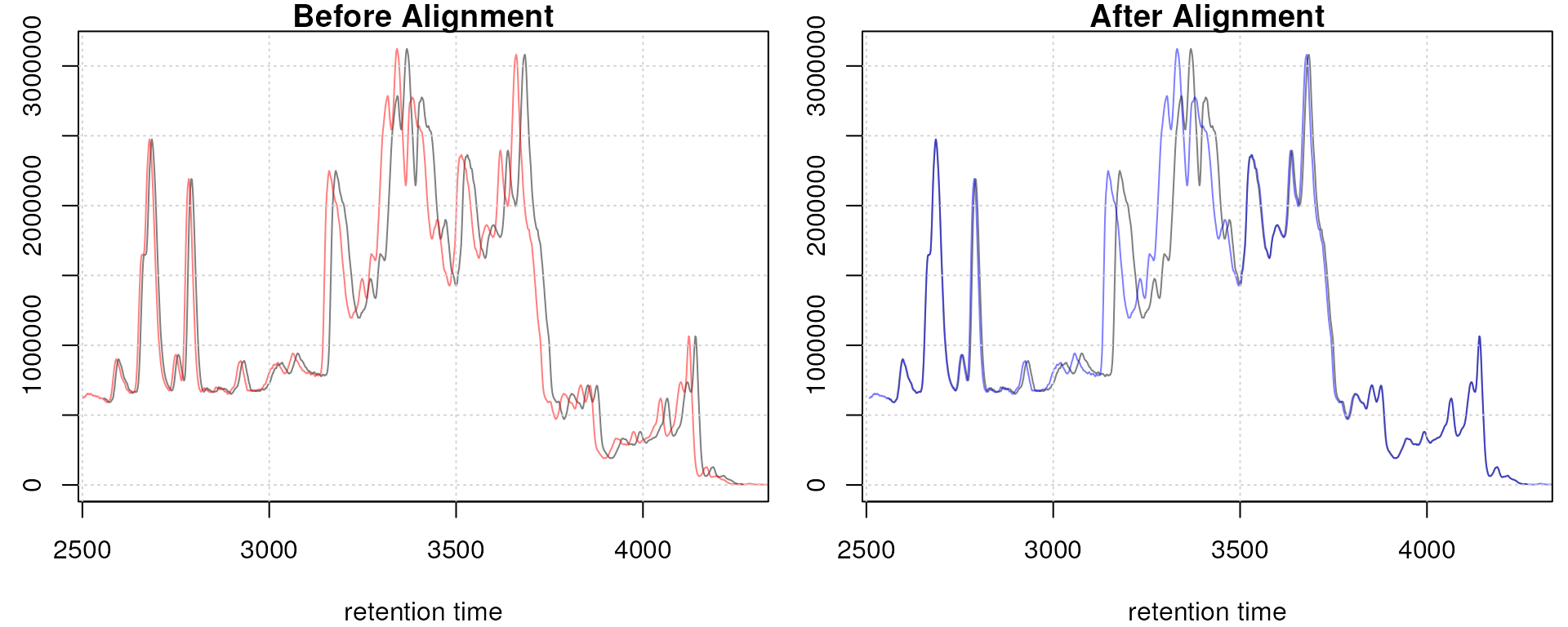
The overlay of BPC above provides insight into the correlation
between accurate alignment and the presence of peaks matching with
lamas. For this particular sample no chromatographic peaks
were matched to the lamas between 2500 and 3000 seconds and
hence the alignment in that region was not good. For the second file,
chrom peaks could also be matched in that region resulting in a better
alignment.
par(mfrow = c(1, 1))
plot(bpc[1, 2], col = "#00000080", main = "Distribution CP matched to Lamas")
points(rtime(bpc_tst_adj[1, 2]), intensity(bpc_tst_adj[1, 2]), type = "l",
       col = "#0000ff80")
grid()
abline(v = mtch[[2]]$obs)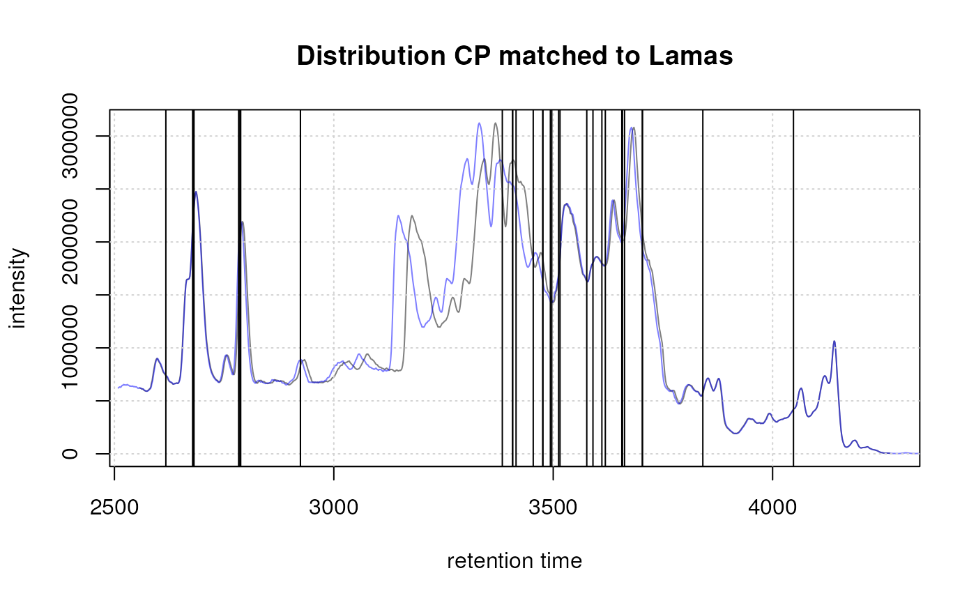
Furthermore, a more detailed examination of the matching and the
model used for fitting each file is possible. Numerical information can
be obtained using the summarizeLamaMatch() function. From
this, the percentage of chromatographic peaks utilized for alignment can
be computed relative to the total number of peaks in the file.
Additionally, it is feasible to directly plot() the
param object for the file of interest, showcasing the
distribution of these chromatographic peaks along with the fitted model
line.
#' access summary of matches and model information
summary <- summarizeLamaMatch(param)
summary
## Total_peaks Matched_peaks Total_lamas Model_summary
## 1 87 34 347 30, c(0.....
## 2 100 51 347 48, c(0.....
## 3 61 34 347 33, c(0.....
#' coverage for each file
summary$Matched_peaks / summary$Total_peaks * 100
## [1] 39.08046 51.00000 55.73770
#' access the information on the model of for the first file
summary$Model_summary[[1]]
## Call:
## loess(formula = ref ~ obs, data = rt_map, weights = weights,
## span = span)
##
## Number of Observations: 30
## Equivalent Number of Parameters: 7.64
## Residual Standard Error: 2.235
## Trace of smoother matrix: 8.45 (exact)
##
## Control settings:
## span : 0.5
## degree : 2
## family : gaussian
## surface : interpolate cell = 0.2
## normalize: TRUE
## parametric: FALSE
## drop.square: FALSE
#' Plot obs vs. ref with fitting line
plot(param, index = 1L, main = "ChromPeaks versus Lamas for the first file",
     colPoint = "red")
abline(0, 1, lty = 3, col = "grey")
grid()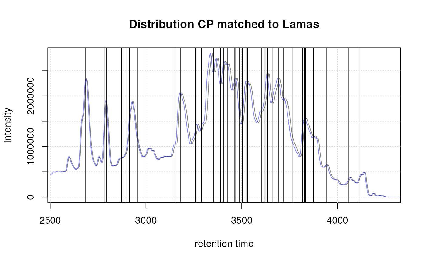
Additional details and notes
Subsetting and filtering
xcms result objects can be subset/filtered by sample using
the [ method or one of the filter* functions
(although the XcmsExperiment supports at present only few
selected filter functions). In some cases filtering can remove
preprocessing results, but most filter functions support parameters
keepFeatures and keepAdjustedRtime that can be
set to TRUE to avoid their removal.
Parallel processing
Most functions in xcms support parallel processing, which is
enabled by default and is performed, for most operations, on a
per-sample basis. Parallel processing is handled and configured by the
BiocParallel Bioconductor package and can be globally
defined for an R session. Note that, while all data objects are designed
to have a low memory footprint by loading only MS peak data into memory
when needed, parallel processing will increase this demand: in general,
the full MS data for as many files as there are parallel processes are
loaded into memory at a time. This needs also to be considered, when the
number of parallel processes is defined. Also, the newer xcms
data analysis functions support the chunkSize parameter
that allows to define the number of data files from which the MS data
should be loaded into memory at a time. This data chunk is then
distributed across the parallel processes. Therefore, the number of
parallel processes should not be larger than chunkSize.
Finally, for very large experiments, the XcmsExperimentHdf5
object should be used which stores all preprocessing results
on-disk in a file in HDF5 format hence further reducing the
memory demand during preprocessing. See the respective example workflow
on Metabonaut
or refer to the ?XcmsExperimentHdf5 help page.
Unix-based systems (Linux, macOS) support multicore-based
parallel processing. To configure it globally we register()
the parameter class. Note also that bpstart() is used below
to initialize the parallel processes.
Windows supports only socket-based parallel processing:
Main differences to the MSnbase-based xcms
version 3
-
Spectrais used as the main container for the (raw) MS data. Thus changing backends is supported at any stage of the analysis (e.g. to load all data into memory or to load data from remote databases). - Support for memory-saving analysis of very large experiments through
the new
XcmsExperimentHdf5object: use parameterhdf5Filein thefindChromPeaks()call to enable this. See also?XcmsExperimentHdf5for more information.
Additional documentation resources
Some of the documentations listed here are still based on xcms version 3 but will be subsequently updated.
- Metabonaut: collection of tutorials and playbooks for metabolomics data analysis in R and beyond.
- Exploring and analyzing LC-MS data with Spectra and xcms: tutorial explaining general data handling using the Spectra package and LC-MS data preprocessing with xcms.
- MetaboAnnotationTutorials: examples for annotation of metabolomics data from [4].
- [2]: describes the concept of the on-disk data modes used also in xcms.
- SpectraTutorials: tutorials describing the Spectra package and its functionality.
Session information
R packages used for this document are listed below.
## R Under development (unstable) (2026-04-19 r89916)
## Platform: x86_64-pc-linux-gnu
## Running under: Ubuntu 24.04.4 LTS
##
## Matrix products: default
## BLAS:   /usr/lib/x86_64-linux-gnu/openblas-pthread/libblas.so.3
## LAPACK: /usr/lib/x86_64-linux-gnu/openblas-pthread/libopenblasp-r0.3.26.so;  LAPACK version 3.12.0
##
## locale:
##  [1] LC_CTYPE=en_US.UTF-8       LC_NUMERIC=C
##  [3] LC_TIME=en_US.UTF-8        LC_COLLATE=en_US.UTF-8
##  [5] LC_MONETARY=en_US.UTF-8    LC_MESSAGES=en_US.UTF-8
##  [7] LC_PAPER=en_US.UTF-8       LC_NAME=C
##  [9] LC_ADDRESS=C               LC_TELEPHONE=C
## [11] LC_MEASUREMENT=en_US.UTF-8 LC_IDENTIFICATION=C
##
## time zone: UTC
## tzcode source: system (glibc)
##
## attached base packages:
## [1] stats4    stats     graphics  grDevices utils     datasets  methods
## [8] base
##
## other attached packages:
##  [1] SummarizedExperiment_1.41.1 Biobase_2.71.0
##  [3] GenomicRanges_1.63.2        Seqinfo_1.1.0
##  [5] IRanges_2.45.0              S4Vectors_0.49.2
##  [7] BiocGenerics_0.57.1         generics_0.1.4
##  [9] MatrixGenerics_1.23.0       matrixStats_1.5.0
## [11] MsExperiment_1.13.1         ProtGenerics_1.43.0
## [13] pheatmap_1.0.13             RColorBrewer_1.1-3
## [15] pander_0.6.6                faahKO_1.51.0
## [17] xcms_4.9.4                  BiocParallel_1.45.0
## [19] BiocStyle_2.39.0
##
## loaded via a namespace (and not attached):
##  [1] DBI_1.3.0                   rlang_1.2.0
##  [3] magrittr_2.0.5              clue_0.3-68
##  [5] MassSpecWavelet_1.77.0      otel_0.2.0
##  [7] compiler_4.7.0              PTMods_0.99.6
##  [9] systemfonts_1.3.2           vctrs_0.7.3
## [11] reshape2_1.4.5              stringr_1.6.0
## [13] crayon_1.5.3                pkgconfig_2.0.3
## [15] MetaboCoreUtils_1.19.3      fastmap_1.2.0
## [17] XVector_0.51.0              rmarkdown_2.31
## [19] preprocessCore_1.73.0       ragg_1.5.2
## [21] purrr_1.2.2                 xfun_0.57
## [23] MultiAssayExperiment_1.37.4 cachem_1.1.0
## [25] jsonlite_2.0.0              progress_1.2.3
## [27] DelayedArray_0.37.1         prettyunits_1.2.0
## [29] parallel_4.7.0              cluster_2.1.8.2
## [31] R6_2.6.1                    bslib_0.10.0
## [33] stringi_1.8.7               limma_3.67.1
## [35] jquerylib_0.1.4             iterators_1.0.14
## [37] Rcpp_1.1.1-1                bookdown_0.46
## [39] knitr_1.51                  Matrix_1.7-5
## [41] igraph_2.3.0                tidyselect_1.2.1
## [43] abind_1.4-8                 yaml_2.3.12
## [45] doParallel_1.0.17           codetools_0.2-20
## [47] affy_1.89.0                 lattice_0.22-9
## [49] tibble_3.3.1                plyr_1.8.9
## [51] S7_0.2.1-1                  evaluate_1.0.5
## [53] desc_1.4.3                  Spectra_1.21.7
## [55] pillar_1.11.1               affyio_1.81.0
## [57] BiocManager_1.30.27         foreach_1.5.2
## [59] MSnbase_2.37.0              MALDIquant_1.22.3
## [61] ncdf4_1.24                  hms_1.1.4
## [63] ggplot2_4.0.3               scales_1.4.0
## [65] glue_1.8.1                  MsFeatures_1.19.0
## [67] lazyeval_0.2.3              tools_4.7.0
## [69] mzID_1.49.1                 data.table_1.18.2.1
## [71] QFeatures_1.21.3            vsn_3.79.6
## [73] mzR_2.45.1                  fs_2.1.0
## [75] XML_3.99-0.23               grid_4.7.0
## [77] impute_1.85.0               tidyr_1.3.2
## [79] MsCoreUtils_1.23.10         PSMatch_1.15.3
## [81] cli_3.6.6                   textshaping_1.0.5
## [83] S4Arrays_1.11.1             dplyr_1.2.1
## [85] AnnotationFilter_1.35.0     pcaMethods_2.3.0
## [87] gtable_0.3.6                sass_0.4.10
## [89] digest_0.6.39               SparseArray_1.11.13
## [91] htmlwidgets_1.6.4           farver_2.1.2
## [93] htmltools_0.5.9             pkgdown_2.2.0.9000
## [95] lifecycle_1.0.5             statmod_1.5.1
## [97] MASS_7.3-65